ML workflow

The problem of autocorrelation is a subproblem of the larger issue of forecasting/predicting when samples are not independent. Most of the ‘easy’ or ‘classical’ algorithms assume that independence.

It’s certainly possible to get around this issue – though I don’t think ensembling by itself would get you there. For classical forecasting like ARIMA, differencing is the usual solution. For cross-sectional regression, you’d look into adding a random effect. If you were trying to use XGBoost, you may have to investigate other solutions as well.

2 Likes

I think this is a serious concern that could extend to XGBoost but XGBoost would not be the worst model. First, it performs feature selection during the training which mitigates the problem to some extent by focusing on features that have the most predictive power.

Also regularization helps mitigate the problem. XGBoost has both L1 (LASSO) and L2 (Ridge) regression. But I don’t have enough experience to say there is not still a problem or that this solves everything.

@Marco there is concern about independence in the training process and not just in the predictions.

At the end of the day, cross-validation can provide an individual answer for members. Individual answers with regard to their factor choices and the models they use.

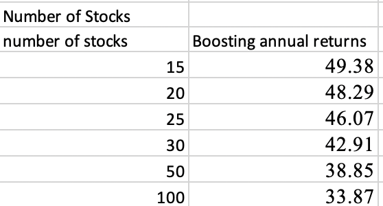
WITH MONOTONIC CONSTRAINTS and cross-sectional data Sklearn’s boosting model does fine (k-fold cross validation with an embargo easy to trade universe). My cross-validation would suggest boosting could be used with some cross-sectional features. No regularization used here (other than early stopping).

And again, I am not sure an embargo solves all of the problem of autocorrelation but it would be worse without it, I think (embargoed k-fold cross-validation):

Screenshot 2024-03-01 at 4.36.19 PM

Jim

1 Like

I would be very hesitant to use XGBoost or any other model on time-based data without some allowance made for violation of independence of samples. As you suggest, cross-validation will be key here. And probably a CV strategy more robust than simply holding out the same 20% of data and testing against that same data 100 times.

I suspect you’d find that your in-sample metrics look great, and the out-of-sample looks awful.

1 Like

Kindly Whycliffes posts some good selection of papers - thanks!

In a lot of them on can find that Random Forest comes out on top.

Is there some experience here that other techniques perform better (boosting, etc.)

I like Extra Trees Regressors best of the ones commonly discussed. I have one that seems to do better (that is not commonly discussed). Support Vector machines run too slowly on my machine to test them and I have not done a neural-net recently or with good factors.

BTW, Extra Trees Regressor (like random forests) doesn’t not have a lot of difficult-to-understand hyperparameters to adjust. It is considered one of the easier machine learning methods to use. Random forests are slow with Extra Trees regressors being much faster.

1 Like

I do get there is an assumption of independence of the independent variable and that this assumption is clearly violated when there is autocorrelation. There can be no doubt of that. Other assumptions are violated too. There is the assumption of i.i.d. data (independent and identically distributed) as I am sure you already know. Market regimes are not identically distributed, I think. I agree. Assumptions are violated. No question.

1 Like

Yes, i.i.d. is another way to say independence of sample. Actually, a smart way to test your cross-validation would be to train a model on unadjusted data and see if the hold out set(s) are much worse than the training set. (If they aren’t, the CV probably needs to be scrutinized.)

There are definitely ways to handle violation of i.i.d. It just adds a wrinkle – most of the simple tutorials you get by googling are no longer applicable.

As I say to clients all the time – ML is not magic! It’s hard! Much more thought and effort is needed than just from xgboost import xgbregressor.

2 Likes

TL;DR: Thank you Pitmaster for bring up the issue of feature autocorrelation. I had previously missed that de Prado was addressing feature correlation here:Advances in Financial Machine Learning with regard to cross-validation. I had been thinking he was talking about the target. But from the text: “Consider a serially correlated feature X…” I am not saying this is the final word and it is only about cross-validation at that. i think you may have broader concerns beyond cross-validation. Maybe my cross-validation methods have benefitted from this discussion.

So we can do some things to improve our models. Many things including addressing issues of autocorrelation. That is a given.

benhorvath says it well here:

I think he is right about that. A wise professor of medicine once said to me: “The reason that there are so many treatment options for this condition is they are all flawed. If there was a really good treatment we would all be using the same one.” Encouraging words indeed as I was about to start a treatment.

Maybe an analogy for the large number of methods published for predicting the market with machine learning. More simply: “It is hard” as benhorvath says.

So I have this question for myself mainly. Knowing I am a flawed individual using flawed methods with limited time to perfect my models is there a good method to test whether my model is reallly better than listening to Jim Cramer on CNBC before I fund it?

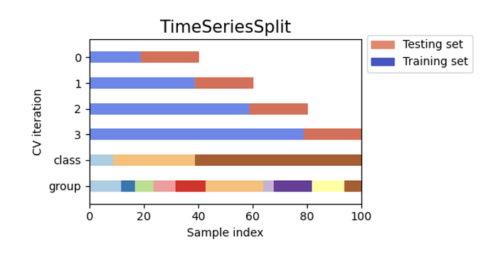
I note when I ask this that there is a method of cross-validation that uses Time Series Split for cross-validation at SKlearn.

It seems it is intended to address—at least in part–this problem: " Time series data is characterized by the correlation between observations that are near in time (autocorrelation )".

I leave it to someone smarter than me to discuss how well the people at Sklearn have done at addressing the problem of autocorrelation with this method. But I did use it before funding my present (not a random forest) model—knowing it would never be perfect. Used it because autocorrection can be a problem, I think. And will continue to look for ways to mitigate the problem in my models and cross-validation of those models.

Addendum (for geeks like me mainly):

De Prado discussed this in dept in the book: Advances in Financial Machine Learning

And excerpt from 7.3 WHY K-FOLD CV FAILS IN FINANCE

Leakage takes place when the training set contains information that also appears in the testing set. Consider a serially correlated feature X that is associated with labels Y that are formed on overlapping data: Because of the serial correlation, Xt ≈ Xt + 1.

de Prado, Marcos López. Advances in Financial Machine Learning (p. 195). Wiley. Kindle Edition. .

One just needs to understand:

  1. Leakage is a bad thing and can be caused by autocorrelation in k-fold cross-validation

  2. Serial correlation is the same thing as autocorrelation in this context.

  3. An embargo used with k-fold cross-validation and also walk-forward cross-validation are proposed as solutions to the problem of autocorrelation in this book.

  4. Bagging as is used in random forest was also proposed as a solution for classifiers at least (de Prado, Marcos López. Advances in Financial Machine Learning (p. 196). Wiley. Kindle Edition.)

Jim

1 Like

Jrinne & benhorvath

Your both quoting de Prado frequently, just thought I’d mention if you already haven’t come across it.

In Github search for “de Prado’, there are several posts where people have replicated code for several of his book examples.

RAM

1 Like

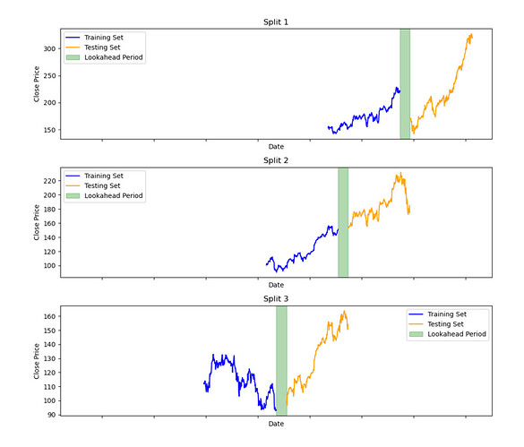
In the book of Stefan Jansen I found a cross-validation method which splits the cross-validation dataset in x-times training, lookout and test.
Basically lookout is used to account for the label, to not mix it later with the test.
This is different from the SKLearn which only uses train and test.

You can as well find his cv function in his GitHub somewhere.

1 Like

TL;DR: I just realized that de Prado is using methods of cross-validation to mitigate the problem of autocorrelation and then going ahead and using machine learning models including boosting. I think that is the most informative piece of information I have.

I edited out my interested in exchageabiliy to replace i.i.d. as an assumption for machine learning as I cannot prove my data is exchangeable.

But if autocorrelation is a concern for de Prado his concerns are constrained and have not stopped him from using machine learning. Maybe he makes adjustments similar to what @pitmaster and @benhorvath make and/or allude to. They have formal training in this area and my understanding is limited. I don’t believe I have a definitive answer. Certainly nothing like a proof about when you can use non- i.i.d. data. Actually, not even a rule of thumb. My understanding is limited and I know that…

I would add this practical consideration. If you use de Prado’s Purge and Embargo method and you use Trailing Twelve Month (TTM) data as one or more of your features, your embargo period (or Purge period) may need to be a year or longer.

I will stop here and get back to my Random Forest models of cross-sectional data for now.—and hope cross-validation of my flawed models helps. I look forward to more-informed opinions and any additional practical methods on this topic.

.

2 Likes

Not sure if it fits into this thread, but the name is ML workflow:

For my workflow I tested some data preprocessing on features.

The first was StandardScaler from scikit-learn, they say:
Quote
Standardization of datasets is a common requirement for many machine learning estimators implemented in scikit-learn; they might behave badly if the individual features do not more or less look like standard normally distributed data: Gaussian with zero mean and unit variance .
End quote

I did not found any effect.
Do I misunderstand something, how is you experience?
Here is the code:

    scaler = StandardScaler()
    
    # Fit the scaler on the training data and transform both training and test data
    # Note: To maintain the multi-index and columns, we operate on the DataFrame values then reconstruct the DataFrame
    
    # Scale X_train
    X_train_scaled_values = scaler.fit_transform(X_train.values)
    X_train = pd.DataFrame(X_train_scaled_values, index=X_train.index, columns=X_train.columns)
    
    # Scale X_test using the same scaler
    X_test_scaled_values = scaler.transform(X_test.values)
    X_test = pd.DataFrame(X_test_scaled_values, index=X_test.index, columns=X_test.columns)

Second attempt should denoise the features, I found it in the book: de Prado, Marcos López . Machine Learning for Asset Managers, Chapter 2.5 Denoising.
Quote
It is common in financial applications to shrink a numerically ill-conditioned covariance matrix (Ledoit and Wolf 2004). By making the covariance matrix closer to a diagonal, shrinkage reduces its condition number. However, shrinkage accomplishes that without discriminating between noise and signal. As a result, shrinkage can further eliminate an already weak signal.
End quote
Maybe I programmed that wrong, it has as well no effect.
If someone has some experience, feedback would be greatly appreciated.
Here is the code:

def cov2corr(cov):
    std = np.sqrt(np.diag(cov))
    corr = cov / np.outer(std, std)
    corr[corr < -1], corr[corr > 1] = -1, 1  # Numerical stability
    return corr

def getPCA(corr):
    pca = PCA()
    pca.fit(corr)
    return pca.explained_variance_, pca.components_.T

def denoisedCorr(eVal, eVec, nFacts):
    # Copy and adjust the eigenvalues
    eVal_ = np.diag(eVal).copy()
    eVal_[nFacts:] = eVal_[nFacts:].sum() / float(eVal_.shape[0] - nFacts)
    # Do not call np.diag on eVal_ again, as it is already a diagonal matrix
    
    # Compute the denoised correlation matrix
    corr1 = np.dot(eVec, eVal_).dot(eVec.T)
    corr1 = cov2corr(corr1)
    return corr1

def denoise(df,d):
    # Handling NaNs and infinite values
    df.replace([np.inf, -np.inf], np.nan, inplace=True)
    df.fillna(0, inplace=True)

    if d > 1:
        d=1

    nFacts = int(round(len(df.columns)*d,0))
    #print('nFacts',nFacts)
    
    # Assume df is your multi-index DataFrame with factors
    corr_matrix = df.corr()
    eVal, eVec = np.linalg.eigh(corr_matrix)
    
    #nFacts = 10  # Example value, adjust based on your analysis
    
    # Denoise the correlation matrix
    denoised_corr = denoisedCorr(eVal, eVec, nFacts)
    
    # Replace infinite values with NaNs
    denoised_corr[np.isinf(denoised_corr)] = np.nan
    # Fill NaNs with zero
    denoised_corr = np.nan_to_num(denoised_corr)

    do_plot = False
    if do_plot:
    
        denoised_eVal, _ = getPCA(denoised_corr)
        
        # Ensure eigenvalues are sorted in descending order
        original_eVal_sorted = np.sort(eVal)[::-1]
        denoised_eVal_sorted = np.sort(denoised_eVal)[::-1]
        
        # Plot the eigenvalues
        plt.figure(figsize=(10, 7))
        plt.semilogy(original_eVal_sorted, label='Original eigen-function', linestyle='-', linewidth=2)
        plt.semilogy(denoised_eVal_sorted, label='Denoised eigen-function', linestyle='--', linewidth=2)
        plt.ylabel('Eigenvalue (log-scale)')
        plt.xlabel('Eigenvalue number')
        plt.title('Comparison of Eigenvalues: Original vs Denoised')
        plt.legend()
        plt.show()
    
    # Initialize PCA with the number of components you found relevant
    pca = PCA(n_components=nFacts)  # nFacts is the number of factors you decided to keep
    pca.fit(denoised_corr)
    
    # Transform the original factors
    transformed_factors = pca.transform(df)
    
    # Perform inverse transform to get denoised factors
    denoised_factors = pca.inverse_transform(transformed_factors)
    
    # Convert denoised factors back to DataFrame
    denoised_df = pd.DataFrame(denoised_factors, index=df.index, columns=df.columns)

    return denoised_df

.

I did as well some tests on the label, again not successful,
now going to enjoy :wine_glass: :joy:
Stuff is difficult

Please see:

Coqueret, Guillaume; Guida, Tony. Machine Learning for Factor Investing: Python Version (Chapman and Hall/CRC Financial Mathematics Series) (English Edition) (S.i). CRC Press. Kindle-Version.

Chapter 4
http://www.mlfactor.com/chap_4.html

from statsmodels.distributions.empirical_distribution import ECDF # to use the ECDF built in function
def norm_0_1(x):
    return (x-np.min(x))/(np.max(x)-np.min(x))
def norm_unif(x):
    return (ECDF(x)(x))
def norm_standard(x):
    return (x- np.mean(x))/np.std(x)

.

Results:
norm_0_1 → no difference
norm_unif(y_train) → worse
norm_standard(y_train) → no difference

Im using a ExtraTreesRegressor.

If someone has some experience with Data preprocessing, feedback would be greatly appreciated - Thankx
@Jrinne ,did not found it.
Could you please point me to the book and chapter, Thanks for pointing out

@Jrinne , your interpretation is due to the autocorrelation, right?
In this case it would be very difficult to react to market changes…that means forget TTM use quarterly only and Purge / Embargo 3 month.

Many but not all ML models require standardization. I do not think standardization makes any difference for a random forest, for example. While I believe standardization is crucial for a neural-net. So a true statment but the devil is in the details.

The book: Advances in Financial Machine Learning

Page number (and heading) here:

WHY K-FOLD CV FAILS IN FINANCE By now you may have read quite a few papers in finance that present k-fold CV evidence that an ML algorithm performs well. Unfortunately, it is almost certain that those results are wrong.”

de Prado, Marcos López. Advances in Financial Machine Learning (p. 195). Wiley. Kindle Edition.

Keep in mind you are only purging or placing an embargo on data AFTER the TEST PERIOD. for your training data.

i was trying to say that if you use TTM you might put an embargo for at least a year AFTER your test data (for your training). BUT you can and SHOULD train on data immediately before your test data. You can capture trends and autocorrelation with the training data just before the test data. But it is not fair to train on data from the same market regime AFTER the test data as your are using information that would not have been available at that time.

Autocorrelation is a complex subject but I think de Prado, at times, does not like to completely remove autocorrelation. For example, he thinks making everything stationary (which removes autocorrelation) removes some information that could be useful. I think you are making the same point in your post.

In other words, you are right. You may not want to remove some of the recent market changes. It is okay to use that if it is before the test data. Can be a good thing but too much may not be good. Pitmaster is correct in that you should at least think about it I believe. For example, maybe not use variables that are correlated to themselves for a year as in his example. That was in interesting example and I think that needs to be considered.

TL;DR: With purging and embargoes De Prado only seeks to remove look-ahead bias or what is often called “information leakage” in the literature. There may be other issues with autocorrelation but he address those elsewhere. For example, he addresses autocorrelation when he discusses making data stationary and is concerned that information is being removed when one does that. Making the subject of autocorrelation complex.

Jim

2 Likes

Jim,
this is my walk forward, please see the picture:

The lookahead is the size of the label, 4 weeks excess return would give a 4 weeks lookahead
Could you please check again, should be ok?

Best
Carsten

1 Like

Keep in mind de Prado does not rebalance (and re-rank with a fresh look at each ticker) everything at a week (or month for monthly rebalance). I think some of what de Prado does is different than what we need to do because of that. HE GETS OVERLAPPING BUY AND SELL SIGNALS THAT MAKE HIS PURGE COMPLEX. More complex than it needs to be for us, I believe.

In any case, no purge or embargo is necessary for a walk-forward cross-validation.

So I think an “embargo” or anything like it is only needed for k-fold cross-validation and not for a walk-forward cross-validation. Also called time-series split over at Sklearn

Sklearn discusses this here: Time Series Split. I think you can lose the green (lookahead period) in your graphic.

For walk-forward you can do this I think (BTW, they are obsessed with that zero-indexing thing). Also note: no rolling window here which is called an “expanding window” or “cumulative” walk-forward validation.

For time-series splits or walk-forward Sklearn does not need to be modified according to de Prado, I believe.

Jim

1 Like

@Jrinne

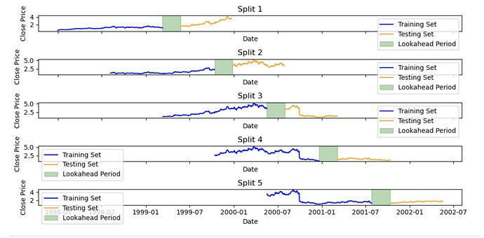
Ok, now starting to understand. This was the original version from the book of Stefan Jansen, can find it at his GitHub.
Orange is train and blue is test.

I thought it had a bug(and changed it for my version).
I think this will avoid the autocorrelation issue at all and it looks like I does not have spill over

Carsten