A method to look at trend following, volatility and correlation for risk reduction without look-ahead bias

Jrinne · April 21, 2025, 10:18am

Geov,

Thanks for weighing in. You make great points about the problems of look-ahead bias and survivorship bias. I agree this is something we should at least be aware of when looking at data.

Question for anyone who’s looked into this more deeply: Does Portfolio Visualizer introduce look-ahead bias? My understanding is that the method itself does not. That it is basically a walk-forward backtest. It uses a 3‑month sliding window walk-forward backtest that does not use any data after the sliding window to change the weightings of the assets. If I’m missing something here, I’d love to understand more.

What I Tested

I ran two strategies using this ETF universe:

TLT, XLB, XLE, XLF, XLI, XLK, XLP, XLU, XLV, XLY

I generally pick these asset to look at sector rotation strategies and because—during some market regimes at least--TLT is inversely correlated to equities. Also it stops me from overfitting by trying different ETFs until I get what I like. And it reduces look-ahead bias to some extent by preventing me from buying assets that I now know have done well in the present, but I would not have known to be the case when the walk-forward backtest was started.

What I’m exploring is a simple question:

Does trend (via recent relative return) improve performance when applied to these ETFs?

Strategy 1: Top 5 Based on 3-Month Relative Return

Each month, select the 5 ETFs with the highest trailing 3‑month return and weight them equally.

Versus:

Strategy 2: Equal Weight Across All 10

Rebalance monthly.

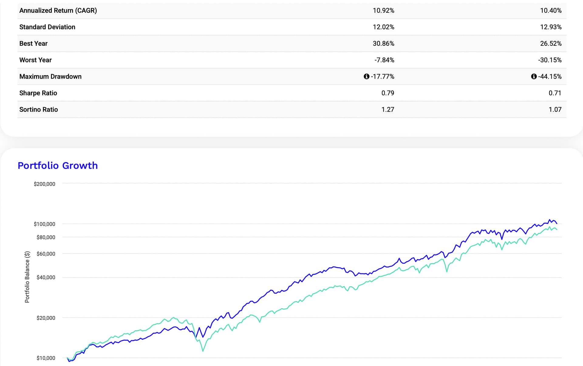
Here’s the result from Portfolio Visualizer:
(Equity curves available if people want to review them directly.)

Adding Volatility Awareness: Risk-Parity Weighting

If we then take the same “Top 5” strategy and weight those 5 ETFs using inverse volatility and correlation of the asset (risk parity equal contribution of risk style), we get improvement in drawdown and risk-adjusted returns (Strategy is the left column and equal weight is the right column):

Key Point

I don’t use either of these strategies myself and certainly this investigation can be expanded. People can draw their own conclusion about the results provided without my comments. But we are able to get some data-driven results about trend-following, volatility, and correlation , I think. Using Python or Portfolio Visualizer for now. What I have done here seems pretty rudimentary but it is real data with reduced look-ahead bias. There is, to be sure, some look-ahead bias in my choice of ETFs which I tried to address to some extent by my ETF selection.

Geov, you make a great point about the problems of look-ahead bias and survivorship bias. I would be interested in your deeper understanding of what strategies work well as you have been doing this for a long time with different strategies and different ETFs.

I would be interested in the direction P123 will be taking when it provides the risk control strategy it is working to provide because, as I say, this is pretty rudimentary even if it does address the question of how market timing can be studied objectively—addressing look-ahead bias by using a walk-forward backtest and sliding window. And how easy (or hard) that can be.

geov · April 21, 2025, 2:39pm

I use the Shiller CAPE divided by its 35-year moving average, CAPE-MA35. Then I smooth it:
short term = 6-month moving average CAPE_MA35_6mo
long term = 240-month moving average CAPE_MA35_240moAvg

Typically, The S&P500 is overvalued when the CAPE_MA35_6mo > 1.45.

• The model uses the CAPE-MA35 ratio to define four phases: Growth, Defensive, Uptrend, and Downtrend.
• Phases are determined by the trend and level of the CAPE-MA35 ratio's 6-month moving average, using linear regression and its position relative to its 20-year average.
• The strategy allocates ETFs based on the phase: Growth (IWF, QQQ), Defensive (XLP, GLD, DBC), Uptrend (DBC, QQQ), and Downtrend (GLD).

Buy rule:
eval($LinRegDownEnter,@downtrend, eval($CAPE_MA35_6mo > $CAPE_MA35_240moAvg & $CAPE_MA35_6mo>1.45 & $LinRegUpEnter,@uptrend, eval($CAPE_MA35_6mo < $CAPE_MA35_240moAvg, eval($CAPE_MA35_6mo<1.35, @Gro,@Gro+@Def), eval($CAPE_MA35_6mo<1.45, @Gro+@Def,@Def))))

Sell rule = 1

From the buy rule one can see that there are periods when the model holds growth and defnesive ETFs at the same time. Thus it is not a binary model, like most market timers. The CAPE is a monthly value, calculated at the last day of the month. For the model I use the PIT value, namely the previous month, because I only update the data series on P123 in the week following the end of the month.

The model shows a positive return for every calendar year since 1999.
In the period to 2025 there are only 57 realized trades - thus very low turnover. The annualized return is over 20%, and the max D/D is only -30%. One can lower the D/D by including a hedge IAU IEF UUP based on the yield curve.

|Total Return|16,078.62%|
|Benchmark Return|579.08%|
|Active Return|15,499.54%|
|Annualized Return|21.33%|
|Annual Turnover|112.69%|
|Max Drawdown|-29.26%|
|Benchmark Max Drawdown|-55.19%|
|Overall Winners|(51/62) 82.00%|
|Sharpe Ratio|1.27|
|Correlation with S&P 500 (SPY:USA)|0.54|

Current holdings are Growth (for 721 days) + Defensive (for 322 days)

pitmaster · April 22, 2025, 4:16pm

Nice results.
Do you compute CAPE in p123 ?

geov · April 22, 2025, 6:16pm

Initially you can download the CAPE data from Shiller at Yale for backtesting. P123 used to have CAPE available but stopped a number of years ago. I do my own calculation in excel. You need the CPI and the average S&P 500 for the month

Calculate the 420 month (35 years) moving average of the CAPE (MA35).
Calculate CAPE-MA35 (CAPE/MA35)
Calculate 6-month and 20-year moving averages of CAPE-MA35

P123 accepts these series from Jan 1970 onward.

See Figure-3 in
https://imarketsignals.com/2025/stocks-are-overvalued-expect-only-modest-10-year-forward-returns-update-march-2025/