TL;DR:
If you form a group, each individual gets to the best solution— MUCH faster than they could by themselves--using the best algorithm available. What more could you ask for?
Background:
Historically, these are called multi-armed bandit problems—think of a row of slot machines (“arms”), each with a different (unknown) payout frequency. You have 500 pulls and keep what you win. Your goal is simple: make the most money possible. To do that, you want to find and pull the arm that pays out best as often as possible—but you need to experiment a bit to discover which one that is.
Thompson Sampling is a proven optimal algorithm for solving this kind of problem: it explores to learn, then exploits to maximize rewards. In real life, Amazon and other companies use similar algorithms for things like testing which web page or ad works best, by showing different users different options and counting “successes.”
For trading, you might use this to find the best trading algo or strategy (e.g., best fill rates)—the idea is exactly the same.
How to use this code:
- Set the true_success_rates list to whatever probabilities you want (these are the hidden win rates).
- Run the code (no seed, so you can see different results each time).
- See how quickly the algorithm finds and sticks to the best arm—visualized and in stats.
Enjoy!
import numpy as np
import matplotlib.pyplot as plt
import seaborn as sns
# Configuration
true_success_rates = [0.10, 0.25, 0.15, 0.40] # True success probabilities
n_arms = len(true_success_rates)
n_rounds = 500
import numpy as np
import matplotlib.pyplot as plt
import seaborn as sns
# Set random seed for reproducibility
#np.random.seed(42)
# Set style for prettier plots
plt.style.use('seaborn-v0_8-darkgrid')
sns.set_palette("husl")
# Set random seed for reproducibility
#np.random.seed(42)
# Configuration
true_success_rates = [0.10, 0.25, 0.15, 0.40] # True success probabilities
n_arms = len(true_success_rates)
n_rounds = 500
# Color scheme
colors = plt.cm.viridis(np.linspace(0, 0.9, n_arms))
optimal_arm = np.argmax(true_success_rates)
# Track successes and failures for each arm
successes = np.zeros(n_arms)
failures = np.zeros(n_arms)
# Track choices and rewards
arm_history = []
rewards = []
cumulative_rewards = []
# Run Thompson Sampling
for i in range(n_rounds):
# For each arm, sample a probability from its Beta distribution
sampled_probs = [np.random.beta(successes[j] + 1, failures[j] + 1)
for j in range(n_arms)]
# Choose the arm with the highest sampled probability
chosen_arm = np.argmax(sampled_probs)
arm_history.append(chosen_arm)
# Simulate pulling the arm
reward = np.random.rand() < true_success_rates[chosen_arm]
rewards.append(reward)
cumulative_rewards.append(sum(rewards))
# Update successes or failures
if reward:
successes[chosen_arm] += 1
else:
failures[chosen_arm] += 1
# Calculate final statistics
arm_counts = np.bincount(arm_history, minlength=n_arms)
estimated_rates = successes / (successes + failures)
# Create figure with subplots
fig = plt.figure(figsize=(14, 8))
gs = fig.add_gridspec(2, 2, hspace=0.3, wspace=0.3, height_ratios=[1.5, 1])
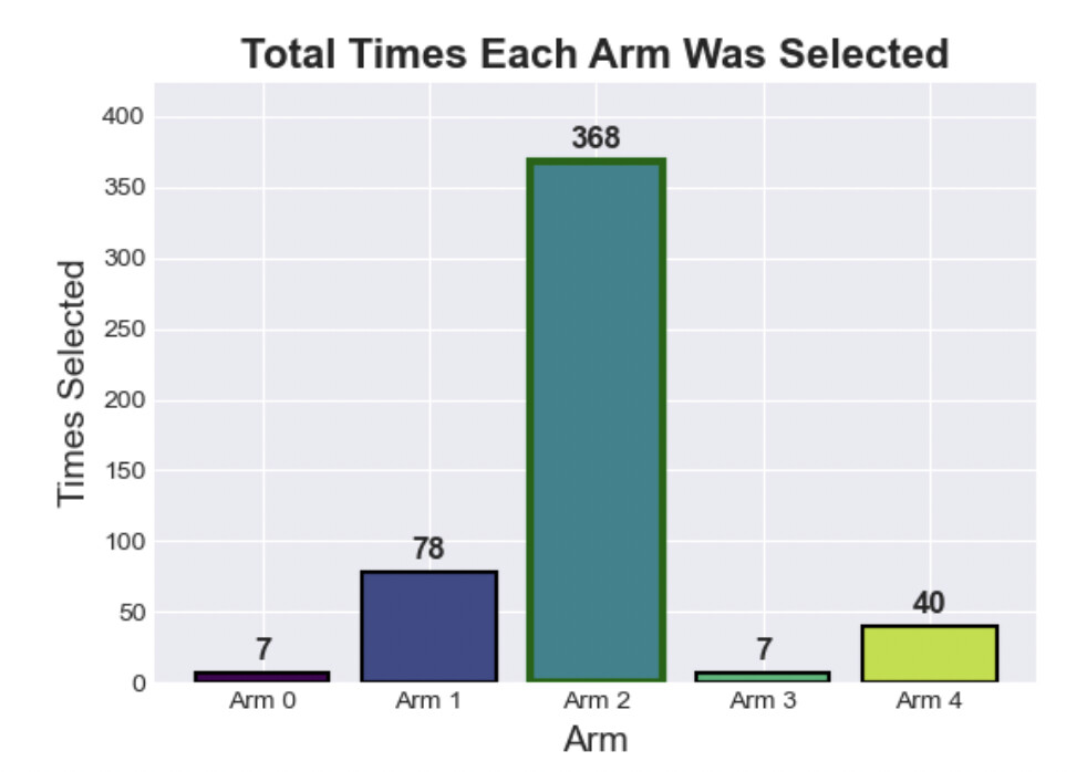
# 2. Total arm selection frequency (top right)
ax2 = fig.add_subplot(gs[0, 1])
bars = ax2.bar(range(n_arms), arm_counts, color=colors, edgecolor='black', linewidth=1.5)
# Highlight the optimal arm
bars[optimal_arm].set_edgecolor('darkgreen')
bars[optimal_arm].set_linewidth(3)
# Add value labels on bars
for i, (count, bar) in enumerate(zip(arm_counts, bars)):
height = bar.get_height()
ax2.text(bar.get_x() + bar.get_width()/2., height + 5,
f'{count}', ha='center', va='bottom', fontsize=12, fontweight='bold')
ax2.set_xlabel('Arm', fontsize=14)
ax2.set_ylabel('Times Selected', fontsize=14)
ax2.set_title('Total Times Each Arm Was Selected', fontsize=16, fontweight='bold')
ax2.set_xticks(range(n_arms))
ax2.set_xticklabels([f'Arm {i}' for i in range(n_arms)])
ax2.set_ylim(0, max(arm_counts) * 1.15)
# 2. Summary statistics table (bottom)
ax3 = fig.add_subplot(gs[1, 0])
ax3.axis('tight')
ax3.axis('off')
# Create table data
table_data = []
headers = ['Arm', 'Times Pulled', 'True Success Rate']
for i in range(n_arms):
row = [
f'Arm {i}',
f'{arm_counts[i]}',
f'{true_success_rates[i]:.3f}'
]
table_data.append(row)
# Create table
table = ax3.table(cellText=table_data, colLabels=headers,
cellLoc='center', loc='center',
colWidths=[0.3, 0.35, 0.35])
# Style the table
table.auto_set_font_size(False)
table.set_fontsize(12)
table.scale(1.2, 1.8)
# Color code the cells
for i in range(n_arms):
# Color the arm column
table[(i+1, 0)].set_facecolor(colors[i])
table[(i+1, 0)].set_text_props(weight='bold')
# Highlight the row of the optimal arm
if i == optimal_arm:
for j in range(3):
table[(i+1, j)].set_facecolor('#90EE90') # Light green
table[(i+1, j)].set_text_props(weight='bold')
# Style header row
for j in range(3):
table[(0, j)].set_facecolor('#4472C4')
table[(0, j)].set_text_props(weight='bold', color='white')
ax3.set_title('Summary Statistics After 500 Trials', fontsize=16, fontweight='bold', pad=20)
# Add main title and key insight
plt.suptitle('Thompson Sampling: Learning Which Arm is Best', fontsize=20, fontweight='bold')
# Add text box with key insight
textstr = f'Key Insight: Thompson Sampling quickly identified and focused on Arm {optimal_arm} (40% success rate)\nwhile still exploring other options. It pulled the best arm {arm_counts[optimal_arm]} times out of {n_rounds}!'
props = dict(boxstyle='round', facecolor='wheat', alpha=0.8)
fig.text(0.5, 0.02, textstr, transform=fig.transFigure, fontsize=14,
horizontalalignment='center', bbox=props)
plt.tight_layout()
plt.show()
# Print simple summary
print("\n" + "="*50)
print("THOMPSON SAMPLING RESULTS")
print("="*50)
print(f"\nAfter {n_rounds} trials:")
print(f"- Best arm (Arm {optimal_arm}) was pulled {arm_counts[optimal_arm]} times ({arm_counts[optimal_arm]/n_rounds*100:.1f}%)")
print(f"- Algorithm achieved {sum(rewards)} total rewards")
print(f"- Average reward per pull: {np.mean(rewards):.3f}")
print(f"- Optimal average would be: {max(true_success_rates):.3f}")
# Calculate what random selection would have achieved
random_expected_reward = np.mean(true_success_rates)
random_total_expected = random_expected_reward * n_rounds
print(f"\nComparison with random selection:")
print(f"- Random would pull each arm ~{n_rounds/n_arms:.0f} times")
print(f"- Random expected total rewards: {random_total_expected:.0f}")
print(f"- Random expected average reward: {random_expected_reward:.3f}")
print(f"- Thompson Sampling improvement: {(sum(rewards)/random_total_expected - 1)*100:.1f}% better!")
print("\nThe algorithm successfully learned which arm was best!")
Key takeaways:
- Thompson Sampling finds and focuses on the best option with remarkable speed and efficiency, while still checking the others occasionally.
- The plots and stats show, at a glance, how well it works.