Factor Momentum

[sthorson]

This is a very interesting discussion. However, it is indeed going in two different directions. It seems to me that the majority view the definition of a factor as macro, i.e. value, sentiment, momentum, etc.

My work focuses on individual factors, 37 to be exact, things like p/s, eps growth, inst%own, p/e, yield, analyst estimate changes and so on.

It is fairly simple, however tedious, to determine which factors are working by using the performance buckets in ranker. Furthermore you can’t just select 10 factors you think are in momentum and then find the stocks with the highest composite rank.

The trick is once you find factors in momentum you must correlate them back to individual stocks. Not at all easy. Simply because yield is in favor it doesn’t mean you just buy stocks with high yield. You must mix the factors so as to blend them into the perfect stock. Having done that, you must then cook up a portfolio that once again blends the factors in favor.

After originating the portfolio you must regularly adjust positions to keep the port in correlation with the natural ebb and flow of the factors in momentum. I do this at the beginning of each month, others I know of prefer quarterly as most of the data is refreshed on a quarterly basis.

I mentioned above the books by Professor Haugen. “The inefficient stock market, what works on Wall Street” is a must read regarding factor momentum, but you should read “The New Finance” first. O’Shaughnessy’s “What works on Wall Street” is also of interest but over simplifies what it takes to truly uncover what’s working now.

I call my buy list the “Superstocks”. If you read Haugen you’ll understand why…

I’ll conclude by adding that factor momentum is just the beginning of my strategy. I also use a bit of MPT and rely heavily on a reward/risk component.

[yuvaltaylor]

This is a very interesting discussion. However, it is indeed going in two different directions. It seems to me that the majority view the definition of a factor as macro, i.e. value, sentiment, momentum, etc.

My work focuses on individual factors, 37 to be exact, things like p/s, eps growth, inst%own, p/e, yield, analyst estimate changes and so on.

It is fairly simple, however tedious, to determine which factors are working by using the performance buckets in ranker. Furthermore you can’t just select 10 factors you think are in momentum and then find the stocks with the highest composite rank.

The trick is once you find factors in momentum you must correlate them back to individual stocks. Not at all easy. Simply because yield is in favor it doesn’t mean you just buy stocks with high yield. You must mix the factors so as to blend them into the perfect stock. Having done that, you must then cook up a portfolio that once again blends the factors in favor.

After originating the portfolio you must regularly adjust positions to keep the port in correlation with the natural ebb and flow of the factors in momentum. I do this at the beginning of each month, others I know of prefer quarterly as most of the data is refreshed on a quarterly basis.

I mentioned above the books by Professor Haugen. “The inefficient stock market, what works on Wall Street” is a must read regarding factor momentum, but you should read “The New Finance” first. O’Shaughnessy’s “What works on Wall Street” is also of interest but over simplifies what it takes to truly uncover what’s working now.

I call my buy list the “Superstocks”. If you read Haugen you’ll understand why…

I’ll conclude by adding that factor momentum is just the beginning of my strategy. I also use a bit of MPT and rely heavily on a reward/risk component.

Hmm. Let’s say that in recent months (or however long your lookback period is) high p/s stocks are really outperforming low p/s stocks. Do you change the direction of your ranking on that factor? Or do you simply change its weight to 0?

[geov]

I programmed the 6-mo smoothed annualized growth rate of a stock or ETF as a custom formula.
I found the formula in a 1999 article published by Anirvan Banerji, the Chief Research Officer at ECRI: " The three Ps: simple tools for monitoring economic cycles - pronounced, pervasive and persistent economic indicators."

Using this growth rate (higher is better) in a one factor ranking system does provide fairly good results for factor ETFs.
I used the iShares ETFs USMV,MTUM,VLUE,QUAL which have an inception date of 4/16/2013. Since the growth formula has a lookback period of 52 weeks one can only start the backtest on 4/17/2014.

Total return was 239% versus 157% for SPY.

The model sold Value and bought Quality on 6/1/2021.

---

[sthorson]

Hmm. Let’s say that in recent months (or however long your lookback period is) high p/s stocks are really outperforming low p/s stocks. Do you change the direction of your ranking on that factor? Or do you simply change its weight to 0?

Yuval, I do none of this in the ranker. Its all coded into custom formula in screener. I have been begging for dynamic weighting in ranking systems for a decade. It would simplify my style in a huge way. Meanwhile I figured out how to do it in screener…

The factors are either outperforming, or they are not. Of the 37 I use, typically 8 - 11 of them are shown to be outperforming at each research cycle. Many are persistent, particularly those factors relating to earnings. So no I don’t flip it’s ranking, if one factor falls off, the portfolio is weighted more toward those factors that are working.

I score every non otc stock based on their mix of the factors in play. So for example if yield has momentum then the stocks are scored based on their place in the deciles of yield. Top decile high score, bottom decile low score. I do this for each factor passing the momentum test. Ultimately each stock is assigned a “Master Score”.

How do I determine which factors are working? I take my universe, and for each factor, a stock will fall into a decile for the factor. Each stock is assigned its 3 month percent return. I then average these returns for each decile. If the top decile average return for a factor is greater than the benchmark 3mo return, the factor passes.

To keep it simple, all factors that pass this test are assigned a weight based on the amount of return over the benchmark. Its heavier than that but you get the idea. And to answer the obvious question “Why not just use the ranker?”, this is impossible to do in ranking, rating, rating pos etc…

[yuvaltaylor]

The factors are either outperforming, or they are not. Of the 37 I use, typically 8 - 11 of them are shown to be outperforming at each research cycle. Many are persistent, particularly those factors relating to earnings. So no I don’t flip it’s ranking, if one factor falls off, the portfolio is weighted more toward those factors that are working.

This is fascinating indeed. Here’s my follow-up question. If a factor’s BOTTOM decile outperforms the benchmark over the last three months, why don’t you switch its direction? Wouldn’t that be more sensible than leaving it out altogether?

Sometimes switching a factor’s direction makes sense. For example, I use net profit margin with lowest numbers best because it’s a great predictor of future earnings growth. And there are times when favoring high beta might be better than favoring low beta (at least in retrospect).

Here’s my next follow-up question. Doesn’t your strategy have enormous turnover if you’re using very different factors and factor weights every month?

Lastly, what brought you to the belief that factors that have outperformed over the last three months are more likely to outperform over the next month rather than reverting to the mean? Have you compared your approach with, say, favoring the factors that have performed well over the last ten years instead?

[Jrinne]

[
Lastly, what brought you to the belief that factors that have outperformed over the last three months are more likely to outperform over the next month rather than reverting to the mean? Have you compared your approach with, say, favoring the factors that have performed well over the last ten years instead?

Yuval,

First, I probably do something more like you do—for now. So I am agnostic on what will work for most members.

But I have looked at what Steve is doing to some extent. He has found something that has worked out-of-sample so I defer to him on most of the answers for what actually works.

But it is pretty easy to test this. Like in this thread: Some Serious Mean-Reversion? . This particular time-period showed mean-reversion. There is always tension between trendng and mean-reversion. And I agree, a year usually shows mean-reversion.

I will say that for my tests 3 months tends to show a positive correlation (trending). And 3 months or 1 month is usually optimal for trending. With 3 months usually being best and with less volatility.

You can do it with the downloads from a sim using Excel, and check several different single factors (in the rank) in about 10 minutes .

Anyway, I think Steve is probably onto something with 3 months and it can be tested easily.

Jim

[Jrinne]

I score every non otc stock based on their mix of the factors in play.

Each stock is assigned its 3 month percent return. .

So, I just want to be clear that I am happy with P123 just the way it is.

Furthermore, I am thankful for Yuval, Marco and everyone at P123 for doing such good work on feature engineering: cleaning up the data, developing fallbacks, making it as PIT as possible, etc.

P123 has a lot of great tools. Full stop. That would include (but not limited to) rank performance, simulations, multiple downloads including the API etc.

Personally, I have been able to use P123’s data, P123’s tools and some outside machine learning methods of my own to develop some ports that are doing well out-of-sample. To be sure, I will want more data on my ports before I claim to have found the Holy Grail of investing.

In summary, thank you P123 and anyone reading this should make sure to sign up and develop their own methods to augment P123’s great tools (if they have not already).

But just an observation: Steve is using the beginnings of machine learning here. He is attaching a set of features (fundamentals over a 3 month period) to each stock and seeing how these affect his target (returns). I am impressed with what Steve has done.

For more about automating this type of thing you should email Steve Auger who is actively doing a lot with Python and Machine learning.

As for P123, if you do not want to see it develop any machine learning ideas, I think you will have to take that up with Marco. He seems to be committed to automating some of this; he uses the term AI.

I look forward to seeing what Marco has developed. But I am completely satisfied with what P123 is doing now.

I would be happy to share my experiences but Steve Auger is a professional programmer and has done machine learning professionally. He has some polished/professional methods. P123 will be providing some ADDITIONAL methods too: in addition to what they already provide.

Jim

[sthorson]

The factors are either outperforming, or they are not. Of the 37 I use, typically 8 - 11 of them are shown to be outperforming at each research cycle. Many are persistent, particularly those factors relating to earnings. So no I don’t flip it’s ranking, if one factor falls off, the portfolio is weighted more toward those factors that are working.

This is fascinating indeed. Here’s my follow-up question. If a factor’s BOTTOM decile outperforms the benchmark over the last three months, why don’t you switch its direction? Wouldn’t that be more sensible than leaving it out altogether?

Interesting question. I suppose it could be found that switching direction might be profitable, but that logic is counterintuitive to my work. The basic premise of my strategy is that “everybody screens”. So the presumption is that their screen will be for whatever the commonly understood best number would be, like low p/e or high yield. My 37 factors are also pretty much top line, commonly searched items.

Here’s my next follow-up question. Doesn’t your strategy have enormous turnover if you’re using very different factors and factor weights every month?

As I’ve mentioned the factors do have persistence, so I’m not flipping the entire portfolio each cycle. I carry 18 - 22 stocks and historically rotate out 3 - 5 each month. Turnover tends to be about 150% annually. Of the 37 factors there is commonly between 6 and 11 that are in favor, and of those about half are already in the mix.

I also have a rule that forces me to not sell until at least 90 days after purchase. Unless of course some event happens. My strategy is a bit leading, so it can take a couple of months for the institutions to find my stocks.

Lastly, what brought you to the belief that factors that have outperformed over the last three months are more likely to outperform over the next month rather than reverting to the mean? Have you compared your approach with, say, favoring the factors that have performed well over the last ten years instead?

Average return of the factor’s top decile stocks is the driver. So to be clear, I’m looking for 3 month outperformance of the factor to tell me what’s working. Then I want the one month factor return to be greater than the three month, this tells me money is flowing into a factor.

Early on my cut off was the factors’ three month vs one year return. This turned out to be a lagging indicator so I stuck with the shorter time frame.

As for ten year lookback my strategy is obviously momentum based, therefore ten years is of no interest. Not to say that ten years wouldn’t work, however if it did everyone would be using it and the factor would be too efficient.

[sraby]

Hello Andreas,

I am interrested to experiment with Factor Momentum. Can you share some of the techniques you used to implement Factor Momentum? You mentionned that you used it as Buy and Sell Rules? What does that look like (from a formula perspective)? Lets say one of your Factor is OpMgn%TTM. How would you impplement Factor Momentum?
Thank,

[judgetrade]

Hey Sraby,
Buy Rule: Rank > 90
Buy Rule: RankPrev(1) < 70

Also on Industry Group Momentum:
FRank(“Close(0)/Close(20)”,#industry,#DESC) > 90 (for example as a buy rule in a model

Best Regards
Andreas

[yuvaltaylor]

Timing equity factors - a good strategy or not? A very nice overview of factor timing research, including factor momentum.

[pitmaster]

I applied Markov process to calculate probability of style outperformance in which the probability of style outperformance depends only on the state attained in the previous event.
In other words the next (day) outperformer depends only on who was the previous (day) outperformer.

As my dataset I used five equity style ETFs from iShares(tickers as name of columns).
In the table below you can see daily returns of these ETFs.
Yesterday (last row) the best performer was the ETF based on SIZE factor ('state' column), 'priorstate' column has value VLUE meaning that it was the best performer a day before.

---

Probabilities of transition from one state to another are shown in the tables below.
For example, the bottom left corner 0.279221 means that if VLUE etf was the best performer yesterday then there is 27.9221% probability that the next day best performer is MTUM etf.

Max values for a row highlighted:

---

Min values for a row highlighted:

---

This is very basic research - more reliable approach would be to use longer period.... but I can provide some conclusions based on daily returns:

• Momentum most often follows (as the winner) the other factors (momentum, size, lowvol, value but not quality).
• The most momentum has Momentum factor (31.77%), the most reversal has Quality factor (12.98%).
• Quality next day outperformance seems to be very random, (not connected to market regime ?)
• The trade with the highest probability of success is to go long MTUM etf if MTUM etf is current winner (31.77%)
• The best long-short trade for next day (1st April 2024) would be to go long momentum (29.8%) and short quality (13.5%).

[ustonapc]

Piotr,

I have my doubts on momentum on different factors but this is very interesting analysis.

Thank you for providing and sharing it with us.

Regards
James

[Jrinne]

Pitmaster,

How would you determine if your results are significant?

I thought a chi-squared test might do the trick as this is a classification problem (categorical variables). ANOVA more suitable for continuous variables.

The actual count is important for the chip-squared test and I did not have that. I am not sure how long each of those ETFs have been in existence. For simplicity I assume 10 years of data (the 2520 in the code is about 10 years of daily data).

Also, I assumed your probabilities reflect true proportions in some sense (theoretical or real) considering the frequentist nature of frequentist statistics.. I am sure I could think of other assumptions that went into this. MOST of them reasonable, I hope. In that regard, I am not sure if the assumption of independence of each ETFs returns on a give day is a major problem or not. Chi-square is a test for independence but not the type of independence I just mentioned, as you know.

This is more of a statistical exercise for me than any attempt to make any decisions (or judgements) about the ultimate usefulness of the strategy or the ultimate usefulness (or optimality) of these particular ETFs if one were to use this strategy. Also note, I probably would not have posted if the results were not significant. Highly significant (p-value < 0.0005). My results are in agreement with your post, I believe.

With these assumptions and with possible errors in my coding taken into account, I get that your results ARE highly significant. Or probably significant in this context—again, I might not have done it just right.

The code and results (expected frequencies cutoff in this screenshot):

[ScottAllenTrading]

Wouldn't this mean that the optimal long-term strategy (sans trading costs) would be to buy MTUM and hold it until a day that QUAL is the top performer, then switch to VLUE for a day, then back to MTUM?

With such a small difference between QUAL->VLUE and QUAL->MTUM though, it seems unlikely that the slight statistical edge would make up for trading costs, meaning... just hold MTUM?

Just to clarify—did you look at Open->Close? Or Open->Open?

[Victor1991]

I was checking out the book mentioned here: Machine Learning for Factor Investing by Guillaume Coqueret and Tony Guida, referenced to by Marco here ML integration Update.

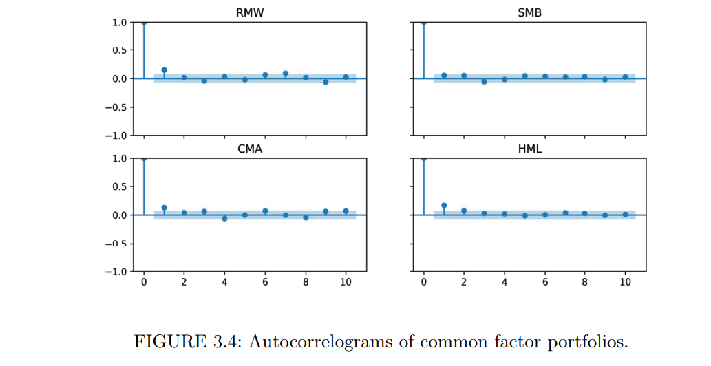
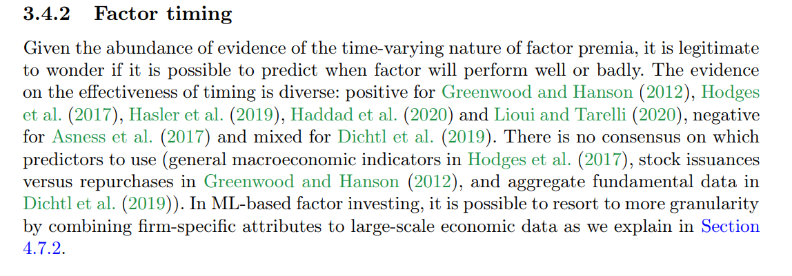
Chapter 3.4.1 and 3.4.2 give a short overview of some recent papers on the subject of factor momentum / factor timing, worth checking out. I've taken two short parts out below.

[pitmaster]

Hi,

I'm using close-close for simplicity...
On the other hand, using this simple analysis, and very liquid etfs, it should be possible to trade close-close, (or near-close).

I also prepared analysis based on weekly data with more etfs.

Interestingly, based on weekly data, when SIZE (small caps) is a prior state, then there is 55% chance that the next state is TLT... but there were only 9 instances of this event between 2013-07-19 - today.
So I'm not sure yet what should be proper trading strategy ...

One of the strategy would be to trade TLT, when prior state was either [SIZE, IVV, QUAL, USVM], otherwise hold IVV. I did a backtest and the results are quite ok but without transaction costs. You may create backtest and confirm my initial findings.

---

DAILY:

---

WEEKLY:

---

Events WHEN SIZE is prior_state:

I used this code:

import yfinance as yf 
import pandas as pd
import numpy as np

tickers = ['IVV','QUAL', 'MTUM', 'SIZE', 'USMV', 'VLUE', 'GLD', 'TLT', 'IWM']

'''Concatenate series returns (close-close) into single df (weekly)'''
data = [yf.Ticker(t).history(period="max")['Close'].asfreq('W-FRI', method='pad') for t in tickers]
df = pd.concat(data, keys=tickers, axis=1).dropna()
df = df.pct_change().dropna()

'''Calculate state and prior state'''
df['state'] = df.iloc[:,-len(tickers):].idxmax(axis=1)
df['priorstate'] = df['state'].shift()
df['cash'] = 0
df.dropna(inplace=True)

'''Create a new DataFrame with only 'priorstate' and 'state' columns, dropping any rows with missing data'''
states = df [['priorstate','state']].dropna()

'''Group the data by 'priorstate' and 'state', count occurrences of each combination, and reshape it into a matrix'''
states_matrix = states.groupby(['priorstate','state']).size().unstack().fillna(0)

'''Convert the frequency distribution matrix into a transition probability matrix'''
transition_matrix = states_matrix.apply(lambda x: x / float(x.sum()), axis=1)
display(transition_matrix.style.highlight_max(color = 'pink', axis = 1))

(if you want prefrom daily analsys just remove this part :".asfreq('W-FRI', method='pad')"

[Jrinne]

Victor,

Edit: I question the significance of just these 2 factors due to the multiple-comparison problem with 40 data points (i.e., none would be significant with the Bonferroni correction). But if you tested 20 different factors and found that all or most had positive correlation for the first few weeks that would be interesting, I think. Maybe use a Fisher's Exact test on 20 factors (categories being 'positively correlated first week' or 'negatively correlated first week'). Just a thought of something that could be looked into. But not enough data in my post for any conclusions, IMHO.

Thank you for that reference. I always like to take the methods of papers and use them with P123 data.

This is the autocorrelation of the excess returns of the top bucket (30 buckets, 2000 - 2024 weekly excess returns relative to the easy to trade universe) for the factors in the screenshot. I leave it to each members to form their own conclusions or test it themselves with their own factors:

Just for those who wish to check my code (or use it). Corrections welcome:

import pandas as pd
import matplotlib.pyplot as plt
from statsmodels.graphics.tsaplots import plot_acf, plot_pacf

(#) Specify the file path (replace with your actual file path)
file_path = '/Users/your_username/Desktop/autocorrelation.csv'

(#) Read the CSV file into a DataFrame
df = pd.read_csv(file_path)

(#) Convert the 'Period' column to datetime and set it as the index
df['Period'] = pd.to_datetime(df['Period'])
df = df.set_index('Period')

(#) Plot autocorrelation and partial autocorrelation with significance bands
fig, axes = plt.subplots(2, 2, figsize=(12, 8))

plot_acf(df['EBITDA / EV'], lags=20, ax=axes[0, 0], alpha=0.05)
axes[0, 0].set_title('Autocorrelation - EBITDA / EV')

plot_pacf(df['EBITDA / EV'], lags=20, ax=axes[0, 1], alpha=0.05)
axes[0, 1].set_title('Partial Autocorrelation - EBITDA / EV')

plot_acf(df['EV to Sales'], lags=20, ax=axes[1, 0], alpha=0.05)
axes[1, 0].set_title('Autocorrelation - EV to Sales')

plot_pacf(df['EV to Sales'], lags=20, ax=axes[1, 1], alpha=0.05)
axes[1, 1].set_title('Partial Autocorrelation - EV to Sales')

plt.tight_layout()
plt.show()

Jim

[yuvaltaylor]

This is not scientific at all, but I thought I'd relate my own anecdotal experience with factor momentum. I broke my factors down into seven general categories and created a way to change their weights depending on factor performance over the last nine months or so. The end result was so much turnover that it seriously damaged my performance.

I came up with an alternative a little while later, and that is to use a few "flip factors" in my ranking system. These are conditional factors that flip between a value factor and a growth factor depending on whether the recent performance of $SPALLPV (S&P 1500 pure value) is better than the recent performance of $SPALLPG (S&P 1500 pure growth). Many of these conditional factors backtest better than either of the included factors alone. This is a very lagging indicator, but because the trends tend to last a while, it seems better than nothing.

[Jrinne]

@Jrinne

But if you tested 20 different factors and found that all or most had positive correlation for the first few weeks that would be interesting, I think. Maybe use a Fisher's Exact test on 20 factors (categories being 'positively correlated first week' or 'negatively correlated first week'). Just a thought of something that could be looked into. But not enough data in my post for any conclusions, IMHO.

I decided to do this with a ranking system that has a modest number of factors most of you would recognize. Many factors are from the core system. You could test this yourself with all of the core system factors or your own ranking system and factors you know and presumably use. You have the code and the P123 downloads to improve on this small study. It could definitely be improved upon but I thought it had enough factors to be interesting.

Modifying the autocorrelation code above, I found 18 out or 31 factors had a positive correlation with a lag of one week. I used the excess returns relative to the easy to trade universe.

Results and code are below. In summary, using 31 factors may not have had enough statistical power, but with 31 common factors I was unable to reject the null hypothesis of no correlation (positive or negative) for the first lag (p-value = 0.15). Also I wonder about the practical significance of only 18 out of 31 factors showing positive correlation for the first lag—over period of 24 years--even if a larger study did show statistical significance.