This is actually one of the reasons I’m working on this project. There’s way too ouch out there that fails to distinguish between (1) tendencies that are attributable to inherent traits of stocks or certain kinds of stocks, versus (2) tendencies that were observed over the course of specific time periods that may or may not have anything to do with the inherent qualities of anything. Bear in mind that empirical stock research is a more dangerous exercise than in many other fields because the available samples tend to be incredibly biased. Due the way things turned out, and skewed by the periods when data became more available, much of what’s available as sample has come from bullish market conditions, and especially in the last 35 years or so, when the market was dominated by plunges in RF which pushed ideal P/E way way way up across the entire equity asset class.
The so-called small cap effect is an example of the second kind of tendency - one that has been observed over the course of specific, but very long - sample periods.
Small per se does not help or hurt returns. The default assumption for small is that Quality is lower, sales and earnings are apt to be more volatile (don’t underestimate what diseconomies of scale – weaker coverage of fixed costs – can do in this regard), and as a result, and stock price are likely to be more volatile. Whether that helps or hurts returns depends on the market’s attitude toward risk taking. The samples used by those who claim to have identified a small cap effect are ones dominated by periods in which the market was good and in which risk taking was rewarded.
Arguably, there is a long-term secular bias toward rising stocks and rewards for risk taking. Population growth, productivity growth, education growth, health care growth, etc. lead to a bias in favor of rising GDP which leads to rising sales, rising profits, etc. So again, we might reason from this to assume a secular tendency toward superior small cap performance.
But when we shrink down to the human investment horizons with which we work, we have to be alert to the potential for periods that will be off-trend, during which small caps will underperform. We might take the patient I’m-not-going-to-try-to-time-this approach as many do, and stick with risk-on/small caps anyway. But at least if you understand the whys and wherefores of small cap performance, you’ll be better able to make sensible decisions whichever way you go, rather than get caught up in the traumas of “Oh my, hs the small cap effect ended?”
I have heard it as: a company cannot expand faster than the GDP for infinity and growth has to eventually equal the GDP (or less).
Put this way the alternative is to believe that the company will eventually crowd out the entire economy. You occasionally see the fantasy nightmare in science fiction movies. A drug so addictive or the price of immortality where nothing else matters. But even here the growth ends up equaling the GDP.
Back to the real world, I do not think even Apple will consume all of our dollars into the future.
Somebody recommended checking Damodaran;s data. He’s pretty good for this sort of thing. My sense, though, is that you may want to take RP up to 4%-5%, which many tend to do (almost as a matter of investment community gentleman’s agreement). And, of course, stay alret for changes in RF.
Also while I like using the 10-year, many many prefer to use the shortest possible Treasury as a proxy for RF since they want to be free not only of credit risk but also market risk.
If you want to keep going along these lines, your next step may be to try to segment the market by size and/or sector and assign different betas for each.
From there, try to identify periods of risk-on versus risk-off and start varying your RP.
As to G, I’d say .02 is the maximum - look for something in line with global population growth perhaps
I do not think you are giving the formula the full credit it deserves. While knowing future growth is hard, as you say, the formula is solid even for plugging in numbers, IMHO. When we give someone money (e.g., our brokers) we want to know how much we will get back (amount and growth of our returns), when we are getting it back (time discount) and the risk that something will happen so we will not get what we expect.
It is all in the formula.
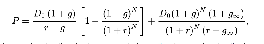
You already mentioned long-tern (non-infinite) growth as a partial solution to the zero denominator problem. But the equation can be expanded for 2 stages (or more) of growth with the latter-stage growth being limited as you describe. See image (source Wikipedia). If you factor in inflation (the real returns) I think a zero denominator is seldom a problem.
Anyway, I think the formula is solid and probably belongs in the core of any sim or port. That is not to say that I don’t believe that a few statistics or backtests cannot help sort out what actually works within the framework of this excellent formula. Thanks for your expertise on this and finance in general!!!
For those who want to see how one advisory company is calculating DCF valuation, including growth rates, risk-free rates, and terminal value, see this web page:
I think parts of this are great and parts are weird. I tried to reproduce this using P123 data but encountered a number of minor difficulties. But it’s an interesting read. Note that the “growth” number they work with has a minimum of 0 and a maximum of 0.2.
Regarding small caps outperforming large caps: I agree with Marc that this is a myth. The average small cap or microcap is more likely to fall dramatically in price than the average large cap. They’re far riskier investments, and so command a risk premium, which is why Marc put size in the “quality” portion of his outline. The advantage small caps and microcaps hold for the savvy investor is that they are more susceptible to fundamental analysis (perhaps they’re less subject to “noise”). See the first two paragraphs of Part II of my article here, along with the chart that follows it:
This is part of the literature, and actually, it’s the bridge that takes us from pure DDM to DCF modeling. You’ll see it referred to as a 2-step, or 3-step, or multi-step approach. Damodaran uses it to value new or less-than-mature businesses.
Again, though, there is the estimation problem . . . and the extent to which the infinite-growth assumption that usually comes at the end influences the final answer.
Can somebody refresh my memory on this: Did the on-line strategy design course cover the RIM (Residual Income Model)? If not, I’ll need to do an add-on. The RIM is a version of DCF that dramatically reduces the number of required inputs and makes for much better credibility than DCF . . . and for which I created a screen on p123.
I said earlier that small caps.as part of the higher-risk lower-quality part of the market, is more prone to do well when the market does well. Yuval’s remarks above are correct and expand on what I said.
Essentially, whatever we’re doing, we’re all looking for anomalies. And because small caps are small, they are in fact easier to grasp and analyze. But nowadays, fewer and fewer people are into serious company analysis so one who does analyze small caps probably has better chances of finding situations where Mr. Market missed the boat . . . maybe underestimating growth, or maybe over-estimating risk (this happens a lot - a risky company priced as if it were twice as risky as it really is makes for an opportunity). The world is so primed by gurus to look for great things, many fail to appreciate how stocks can move if a company goes from ridiculously in the red to just plain in the red, and if they start to get within hailing distance of breakeven, you’ll probably get to take nice profits selling to latecomers bidding the stock up to excessively optimistic levels.
So there’s really nothing wrong with small cap investing, as long as we understand what it is. We’re not naively assuming there’s a “small cap effect” that automatically boosts returns and driving ourselves crazy at times when it seems to vanish. We’re looking for the usual set of V-G/S -Q anomalies and looking in a place where a particular pattern of these anomalies is apt to happen a lot.
A lot of you are already doing this V-S/G-Q type of strategizing it so what I’ve bene writing isn’t meant to get you to change. For folks like you, it’s meant to put some intellectual armor around what you’re doing and helping you stay the course and resist so much nonsense that’s out there.
My mathematical “abilities” limit me to small parts of this, but I do know that although the normal distribution is assumed for just about everything that has come out of financial research, it’s now pretty well acknowledged that in the real world, none of the observed distributions are normal. Third and fourth moments tend to be high, and often the forth moment can be especially notable. I saw that a lot some years ago when I studied many of the factors we use here.
I don’t have the mathematical vocabulary to explain myself, but the Merton model comes from a completely different theoretical heritage.
FWIW, for your own personal use you are likely to be okay using a normal distribution as the central limit theorem saves you most of the time. If you use longer holding periods you are better off using the natural log of the returns. This gives a nice bell shaped, pretty symmetrical curve (usually), that is considered (or assumed to be) lognormal. However, the tails may (or may not) be fatter than a normal distribution.
Merton (Black-Scholes) assumes a lognormal distribution, I think. And again this does work for a big part of what we do—fat tails or not–because of the central limit theorem.
Fat-tails and non-normal distributions are important for leverage, as we all know. We don’t need to read “The Black Swan” buy Nassim Taleb to know this. You know the history and experience where the CAPM has failed (especially with excess leverage) better than I do. Nassim Taleb (and others) have used Long-Term Capital Management as an example—to the point of literally advocating the rescinding some Nobel Prizes. I would be interest in your experience and take on this.
But assuming a fat-tail does not cause you to go broke, over a long period your average returns will be part of a lognormal sampling distribution (central limit theorem).
And as you say it is a different topic. The DDM is, as you suggest, pretty universal. No one gives up money without expecting more money in return. And the sooner they get the money the better (time discounting). The riskier things are (or if they can get almost as much return risk free) the less likely they are to give up their money. The way you present it you successfully extend the theory into discounted cash flow analysis.
That may be the canonical view, but the two are linked by the time value of money principle. The difference is that the Merton model supposes the investor receives a one-time terminal payout of the expected Max(0, FV_Assets - FV_Debt) at maturity where FV_assets is a diffusion process determined by the expected PV of cash flows (or earnings). DCF presupposes that the investor receives NPV of equity over regularly spaced intervals (or continuously) with no diffusion taking place. The chief advantage of DCF is the presumption that earnings accrue discretely, which is a more realistic way of modeling how things work in the real world.
While most DCFs presume no diffusion, it can be shown that the randomness vanishes in the case of DCFs under some unconditional probability measure,
(as this example shows). But conditionally, as in the real world, equity investors actually expect to receive payout Max(0, FV_Assets - FV_Debt) due to the limited liability clause of equity. This would explain why markets assign negatively earning companies positive values… not necessarily because of positive future expectations, but because losses are limited to principal invested. One could think about this residual value as “extrinsic value”.
Not to get lost in weeds, I just was wondering if anyone had though about to how deal with uncertainty of cash flows and how this could affect NPV. As I think I have shown, the embedded “optionality” of equity ensures that equity NPV is at least equal to the unconditional expectation given by DCF. Instead of looking at this uncertainty problem holistically, conventional financial analysis has devised a multitude of ways to price around actual cash flows by evaluating companies by EBITDA, sales, book value, all sorts of variations around interest rates, and more. Not that these are necessarily wrong, but just really rough approximations. Merton-like models are a step the right direction, but are ultimately worse at predicting returns than much simpler cash flows and earnings based perpetuity models (such as what Marc proposes) or structured annuity models (such as what Jim has outlined) since they assume only a one-time payout at maturity (furthermore… what maturity? What drift? What variance? What initial value? etc.).
Anyway, my intuition strongly tells me that an ability to model the conditionality of equity would in turn allow us to more price things under a single framework, meaning fewer assumptions and thus more robust estimates.
There are people who do research in areas like this. You may want to go to web sites for “Journal of Finance,” “Journal of Portfolio Management,” “Financial Analyst’s Journal,” etc. and look at the indexes of published artices (these will be academic research papers). If you see something that catches your attention, Google the name of the article; someone somewhere may have uloaded a opdf you can easily retrieve. If not, you can see how muchb the publication charges for individual-articile access . . . Or try to communicate directyl with the author, who can usually be traced via his or her academic affiliation.
My problem in using sentiment as a factor is one of implementation.
The only effective use, that I have seen, is to look at changes in estimates over the last four to eight weeks. (As used in the Basic ranking system.)
I find using this to give very high high turnover with losses caused by slippage and commissions.
I have played around with other rules that use estimates but none seem to have much effect.
Anyone have any sentiment rules that are effective in lower turnover systems (say 100-300%/yr?)
I like P123’s Basic Sentiment rankings a lot, and use them, but you’re right, that’s for high-turnover systems. For lower turnover systems, try a combination of SI%ShsOut, compared to industry, lower numbers better, and Pr52W%ChgInd, compared to universe, higher numbers better.
David, I don’t know if this counts as sentiment, but there may be a use for longer term comparisons comparing the current analyst estimate to estimates that came before it. For example: CurQEPSMean vs. EPSActual(3,QTR) and permutations of that idea. That would give a longer window of comparison anyway that might be a bit more stable.
I think there’s some effectiveness in various comparisons of that nature and that’s one branch of a new growth model I’m working on. But I’m not sure if it’s strong enough to survive combination with other factors. I’m not to that point yet.
The paper is a high-level description of the Vacicek-Kealhofer model, which is Moody’s proprietary extension to the Merton model. A few years old, but I think it’s a nice conceptual overview.
I am reading now. It does offer a wonderful overview. Thank you.
But I still find the Merton framework circuitous (a chicken and egg ordeal).
How does it value assets? By inverting the market value of debt and equity…
How does it value equity? Through the imputed value of assets…
It assumes that assets are a diffusion process (which is just a modeling assumption), but it does not directly estimate any values provided that their is a market for them. This of course presumes semi-strong form market efficiency – i.e., the market gives the right values for equity and debt. This might be useful to ratings people who guess at credit worthiness or credit portfolio managers, but it says nothing about future equity returns which is what we care about. Also the veracity of this model seems to be antithetical to the existence of risk takers and arbitrageurs such as ourselves.
DCFs, on the other hand, directly impute generic asset values, which is much more strongly aligned to our incentives. Even if markets are usually right, it pays to find out when/where they are wrong. I just keep finding that the existing literature on real options involving DCFs is incredibly lackluster.
Again, the two are linked by time value, but Merton/KVM assumes only a terminal payoff. This is true even if we were to adapt Merton for estimated asset values and (American style) early exercise.