For ML Feature Selection, Can a Larger MSE Actually Mean a Better Model?

@pitmaster reminded me about make_regression. It creates features for which you can control the number of informative (non-noise) features, correlation of the feature and the global amount of noise in the data.

I thought I would use it to answer questions like "How many noise factors can I add before ExtraTreesRegressor stops working?" I am not sure I can simulate stock data exactly but at least I know which are the noise factors and how may of them there are with make_regression as I can control that. That question was kind of interesting.

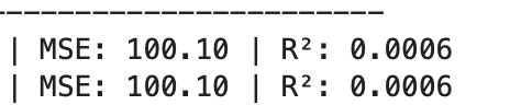
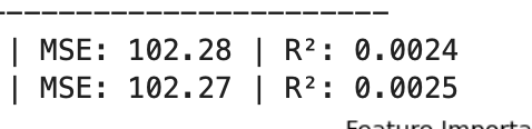
What was unexpected is that when I made more features informative the MSE increased (generally a bad thing)!!! While the R^2 increased (generally good). So contrary indicators with the MSE being suspect as it got worse when more features were informative.

MSE and R^2 for 2 models I was checking out with 10/50 informative features:

Screenshot 2025-08-07 at 12.45.31 PM

Now with 40/50 informative features:

So question:

  1. Will MSE give you a false impression--at least when you are trying features? Honestly this is new and I am not sure how to interpret this. ChatGPT had some ideas but you can go to ChatGPT directly.

  2. Is make_regression useful to us? And if so how.

I was comparing 2 models that Yuval and Pitmaster were recommending. Pretty much a tie (with these parameters) so maybe ignore that. If it was not a tie I probably would have modified the code to avoid getting sidetracked. I am just interested in the above questions.


import numpy as np
import matplotlib.pyplot as plt
from sklearn.datasets import make_regression
from sklearn.ensemble import ExtraTreesRegressor
from sklearn.model_selection import train_test_split
from sklearn.metrics import mean_squared_error, r2_score

# ----------------------------------------
# 1. Generate synthetic regression data
# ----------------------------------------
X, y, coef = make_regression(
    n_samples=100_000,          # scaled down for speed
    n_features=50,
    n_informative=40,
    effective_rank=10,          # adds correlation structure
    noise=10.0,
    coef=True,
    random_state=0
)

# ----------------------------------------
# 2. Train/test split
# ----------------------------------------
X_train, X_test, y_train, y_test = train_test_split(
    X, y, test_size=0.2, random_state=1
)

# ----------------------------------------
# 3. Define Yuval's model
# ----------------------------------------
model_yuval = ExtraTreesRegressor(
    n_estimators=100,
    max_depth=8,
    min_samples_split=2,
    #min_samples_leaf=100,
     max_features = 0.3,
    random_state=42,
    n_jobs=-1
)

# ----------------------------------------
# 4. Define Pitmaster's model
# ----------------------------------------
model_pitmaster = ExtraTreesRegressor(
    n_estimators=100,
    max_depth=None,
    #min_samples_split=2,
    min_samples_leaf=500,
    max_features = 0.3,
    random_state=42,
    n_jobs=-1
)

# ----------------------------------------
# 5. Fit and evaluate Yuval's model
# ----------------------------------------
model_yuval.fit(X_train, y_train)
y_pred_yuval = model_yuval.predict(X_test)
mse_yuval = mean_squared_error(y_test, y_pred_yuval)
r2_yuval = r2_score(y_test, y_pred_yuval)

# ----------------------------------------
# 6. Fit and evaluate Pitmaster's model
# ----------------------------------------
model_pitmaster.fit(X_train, y_train)
y_pred_pitmaster = model_pitmaster.predict(X_test)
mse_pitmaster = mean_squared_error(y_test, y_pred_pitmaster)
r2_pitmaster = r2_score(y_test, y_pred_pitmaster)

# ----------------------------------------
# 7. Print comparison
# ----------------------------------------
print("Performance Comparison:")
print("-" * 40)
print(f"Yuval's Model     | MSE: {mse_yuval:.2f} | R²: {r2_yuval:.4f}")
print(f"Pitmaster's Model | MSE: {mse_pitmaster:.2f} | R²: {r2_pitmaster:.4f}")

# ----------------------------------------
# 8. Optional: Plot feature importances
# ----------------------------------------
plt.figure(figsize=(12, 4))
plt.bar(range(50), model_pitmaster.feature_importances_, alpha=0.7, label='Pitmaster')
plt.bar(range(50), model_yuval.feature_importances_, alpha=0.7, label='Yuval')
plt.title("Feature Importances (Comparison)")
plt.xlabel("Feature Index")
plt.ylabel("Importance")
plt.legend()
plt.tight_layout()
plt.show()

# Show the true coefficients
print("True coefficients (non-zero features):")
for i, c in enumerate(coef):
    if abs(c) > 1e-5:
        print(f"Feature {i}: {c:.4f}")

Well if one is real and one is not does it matter? Error could be zero but if it is false data it might not exactly work well in practice. Maybe I am misinterpreting the issue. I would argue real data is better even if MSE is larger since it will of course be more reliable in practice.

TL;DR: Should we use MSE for feature selection?

Some of us might already be doing this — removing features one by one and checking whether the Mean Squared Error (MSE) improves. If it does, we drop that feature and move on. Seems reasonable, right?

After all, a lower MSE means smaller average prediction errors, so the model must be getting better… right?

Well — maybe not.

In my testing, I found something unexpected: MSE increased even as R² improved.

R² measures how much better the model is compared to simply predicting the mean, so it captures a different aspect of model performance. I always understood this in theory — but I didn’t realize how much it could matter in practice. Here, the two metrics led to different conclusions about which model was better.

I’m still wrapping my head around it. But this much seems clear:

The choice of metric can meaningfully affect your decisions during feature selection.

And that’s something I hadn’t fully appreciated — until now.

The way I take it intuitively is the more random stuff you add the more random the behavior of the branches will be and the leaves will look more and more similar (bad r2).

Nice. I like that explanation.

1 Like

Picture a random scatterplot

This does bring up a question though. The scale of the variance matters. There could be situations were error is larger but so are returns. I.e are you trying to predict performance or are you trying to make a killing.

In other words we probably want to penalize downside error more than upside error. Upside error is extra gain but also extra variance😬

I think there must be some bias involved — maybe even a classic bias-variance tradeoff.

R² tells us how well the model captures the direction of the signal, but that doesn’t mean it’s unbiased. Think of a linear model where the slope is correct, but the intercept is way off — directionally useful, but still biased.

MSE, on the other hand, reflects average squared error, which is more sensitive to variance. A model that simply predicts the mean of y for every input would have low MSE (low variance), but it wouldn’t capture any signal — so it would have low R².

So if your goal is to rank stocks or identify winners, even if your return estimates are biased or noisy, then R² might be the better metric.

1 Like

I think my ideal would be to look at something like that (but better) plus downside error. Once I get to testing I will have to learn a lot on different ways to asses. I am stuck on formula and data cleaning and some feature engineering right now.

1 Like

Sounds like you have discovered two well-known facts in ML:

  1. R^2 always increases when you add features.
  2. The bias-variance tradeoff.

Both facts are worth your attention.

R^2 always improves when you add features. This a well-known feature of R^2, and resulted in the creation of adjusted R^2. However, many ML practitioners will recommend you avoid R^2 (or even adjusted R^2) altogether!

As for MSE: When you add features to a model, you are increasing model complexity. Your MSE may improve up to a point, and then the model will become overly complex and MSE will decline (assuming you're not changing anything else, like regularization parameters).

A set of data can only support so many features. You can't have, e.g., 1000 rows and 1,000,000 features. I mean, you can, but usually you use regularization or feature selection or dimensionality reduction to drastically reduce it.

The core finding of ML is the bias-variance trade-off. I highly recommend you study this and internalize it if you're going to use ML, it is directly related to your question.

Finally, I would advise that you consider if MSE is the correct metric for your task. If you are modeling returns, there are probably better metrics/loss functions.

1 Like

Thank you so much — this is helpful and well-said.

I do understand much of what you’ve said, but I was still shocked to see MSE actually increase with a model that was clearly better at ranking stocks. I’ve always known MSE might not be the best choice, but it was eye-opening to see just how misleading it can be — not just suboptimal, but potentially pointing in the wrong direction.

For my downloaded models, I already use a different metric entirely. But I’m increasingly concerned that P123’s grid search may still rely on R² — especially since there’s no clear documentation on what metric is actually being used.

Given that scikit-learn defaults to R² for regression problems, I suspect P123 may be inheriting that default — which, as you’ve articulated well, is far from ideal for ranking problems like ours.

I have been thinking I might have to create some custom formulas to evaluate- if I can find a way later. Learned about huber loss and mean absolute error which seem to work better than mse per the literature but I still think they are terrible for what we are trying to do.

1 Like

What metric/functions would you favor?

I think at the very least I would want mae for gains and mse for losses. Quadratic penalty for negative errors/losses linear penalty for positive errors/gains

I use a couple of different metrics. One of my main tools is to treat the model like a screener. I’ll change a parameter, train the model with that setting, and then use it to rank and select stocks on the validation set — just as a screener would. That effectively turns the screen itself into the evaluation metric, giving me a direct view of what actually matters: how well the model selects stocks in practice.

To avoid overfitting, I don’t screen for just a small number of stocks — though of course, everyone has their own definition of ā€œsmall.ā€ In fact, the number of stocks in the screen could even be treated as a hyperparameter in a grid search — likely a better approach than settling on any single number of stocks.

Since P123 is fundamentally rank-based, Spearman’s rank correlation is an obvious and sensible metric to try. But while it rewards good ranking, it ignores magnitude — and sometimes you want to catch a few large outliers. So while Spearman’s rho makes a lot of sense, it’s not my personal favorite.

That said, just about anything is likely better than using MSE or even R² in this context.

There has also been a lot of interest in "rank:ndcg" — which optimizes NDCG (Normalized Discounted Cumulative Gain) — for XGBoost, and in the equivalent ranking objective for LightGBM. It’s conceptually similar to Spearman’s rank correlation but allows you to prioritize getting the top-ranked stocks right. That’s an appealing property for most use cases in stock selection.

Of course, the default in XGBoost is still "reg:squarederror", which (unfortunately) means you’re back to optimizing MSE unless you override it. If you’re interested in "rank:ndcg", you’ll probably need to download the model and do some extra setup — but it’s worth the effort if you care about ranking performance.

2 Likes

I'm shocked to hear sklearn defaults to R^2 for regression. I would never have guessed that.

The loss function is a crucial part of the entire process, hopefully they'll give you folks an option for that soon.

For more on the perils of R^2, I highly recommend starting at p. 180 here: The Truth About Linear Regression

R^2 does not measure goodness of fit... R^2 can be arbitrarily low when the model is completey correct... R^2 can be arbitrarily close to 1 when the model is totally wrong... R^2 is also pretty useless as a measure of predictability...

For predicting returns, I tend to use spearman_correlation(y, y_hat), which I picked up from a couple papers. This is because I don't really care about estimating the return precisely, all I'm really interested in is ranking. (Note that while Pearson correlation and R^2 are related, this is not the case for Spearman correlation.)

In my experience -- and yours may vary -- optimizing for Spearman correlation has worked well. There are other ways to perform ranked ML, too.

2 Likes

Yes a friend of mine from the site recommended spearman. Good to hear

Interesting one to check out

1 Like

Outside of ML altogether, I use R^2 for determining transaction costs. Given 3 variables, I want to find the best line that explains transaction costs, so I adjust the multipliers of the three variables to maximize R^2 with the line running through the point (0,0), which is a pretty simple process using the solver in Excel. What's wrong with that? Why is R^2 "useless" in this case? I always end up with a line that's a much better fit if I do this.

As usual, experience varies.

For me, I would always prefer to use MSE/etc. R^2 just has so many caveats and oddities that I don't bother with it. (Some of them detailed in the textbook I linked.)

Indeed, forcing the intercept to 0 improve R^2 is one of those well-known oddities. Here is a situation where forcing the intercept to 0 gets a better (reported) R^2, but actually creates a worse model!

|                | R^2 reported | R^2 manual | MSE    |
|----------------|--------------|------------|--------|
| With intercept | 0.799        | 0.799      | 7.810  |
| Zero intercept | 0.956        | 0.692      | 11.973 |

R code:

set.seed(1)

# Simulate data
n <- 100
x <- runif(n, 0, 10)
y <- 5 + 2 * x + rnorm(n, mean = 0, sd = 3)

# Fit with intercept
fit_int <- lm(y ~ x)

# Force to 0
fit_zero <- lm(y ~ x + 0)

# Reported R^2 by summary()
r2_int_reported  <- summary(fit_int)$r.squared
r2_zero_reported <- summary(fit_zero)$r.squared

# Manual R^2 computed about the mean: 1 - SSE / SST(mean)
sse_int  <- sum(resid(fit_int)^2)
sse_zero <- sum(resid(fit_zero)^2)
sst_mean <- sum((y - mean(y))^2)
r2_int_manual  <- 1 - sse_int  / sst_mean
r2_zero_manual <- 1 - sse_zero / sst_mean

# MSE (mean squared error) for each model
mse_int  <- mean(resid(fit_int)^2)
mse_zero <- mean(resid(fit_zero)^2)

comp <- data.frame(
  Model = c("With intercept", "Through origin"),
  R2_reported = c(r2_int_reported, r2_zero_reported),
  R2_manual_about_mean = c(r2_int_manual, r2_zero_manual),
  MSE = c(mse_int, mse_zero)
)
print(comp, row.names = FALSE)