How harmful is optimization?

I decided to run a little experiment. I took some old ranking systems that I had created, ranging from the very first one that I used in December 2015 up to the one I started using in August 2017. During that entire period I was engaged in optimizing my ranking systems by backtesting them.

I created a universe that was typical for my backtests. It had a minimum liquidity of $40,000 median daily total and a minimum market cap of $30 million, excluded MLPs and REITs, excluded stocks from countries with a high corruption index, and excluded stocks with stale statements or M&A activity.

The simulation was also typical. It uses variable slippage, buys the top 20 stocks, and holds them until their rank position is greater than 45; but it doesn’t sell a stock unless it’s been held for at least three weeks.

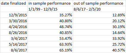
I then ran each ranking system in the order that it was finalized on two periods: an in-sample period of January 1999 to December 2015 and an out-of-sample period from August 2017 to today.

I expected the results to show that the earliest ranking system would have performed the best and the latest the worst because of the ill effects of optimization.

But what I found, to my surprise, was the exact opposite. The correlation between in-sample and out-of-sample performance of these seven ranking systems is 0.82.

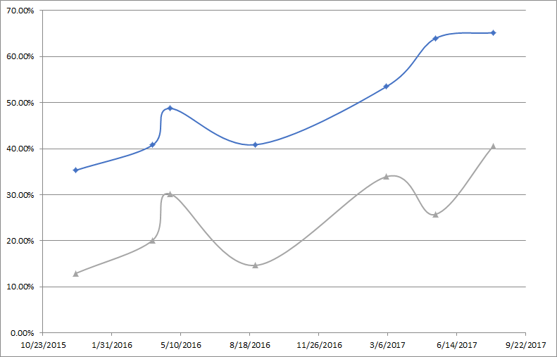
Here are the results (all of them in terms of annualized returns). The blue line is the in-sample return and the gray line is the out-of-sample return.

I’m curious to hear your comments.


is-oos 1.png


That’s a wide range of oos results. Do you feel like your models changed that much with each iteration, or is it a case of slightly different models producing significantly different results?

Hi Yuval,

Thank you!!!
Not sure I get it. Is the blue line the optimized version OOS?

If not: Can you show the results of the not optimized version of the system, that would give a hint if optimization did help with the OOS Performance.
The OOS Performance is a bit short, 2017 - today was a pretty difficult market…

How did you optimize?

Best Regards

Andreas

I enjoy your articles Yuval! I just want to confirm if my understanding is correct:

The rightmost column is annualized OOS result for the ranking system created on the leftmost column date.

In which case the OOS results are of different duration for each date. Am i understanding this correctly. Also, to get a feel for he complexity, how many factors are used?

I guess I wasn’t clear enough.

The models did change quite a bit. The very first model I used was an 11-factor model; by 2017 I was using a 34-factor model and including about double that number in my testing.

The blue line is the optimized version IN sample. The grey line is the out-of-sample results. You see that they correlate pretty well.

I optimized by backtesting, backtesting, backtesting, and adjusting the factor weights according to performance. I used an incremental method, reducing the weight of one factor and increasing another.

The rightmost column presents out-of-sample results only for the period 8-6-17 to 2-5-20. It does not give out-of-sample results for the period between the finalization of each ranking system and 8-6-17 because those wouldn’t really be comparable.

Thanks Yuval.

I am a bit curious about the average annual excess return for insample and then the excess return for each year thereafter. I am curious if there is higher excess returns immediately following the IS period followed by alpha decay or it is is fairly consistent.

A quick and dirty method would be to use a 100% hedge of a comparable benchmark when running the simulator and just make a note or put a mark when it turns out of sample.

It may be that your more recently optimized models perform better simply because of the shorter gap between when the model was optimized and the reported returns.

Kurtis, this is a very good point indeed, and one that hadn’t occurred to me. What I can do, I think, is to get the 30-month alpha subsequent to the end of the in-sample period, using the universe as a benchmark. Maybe that will make the results more comparable.

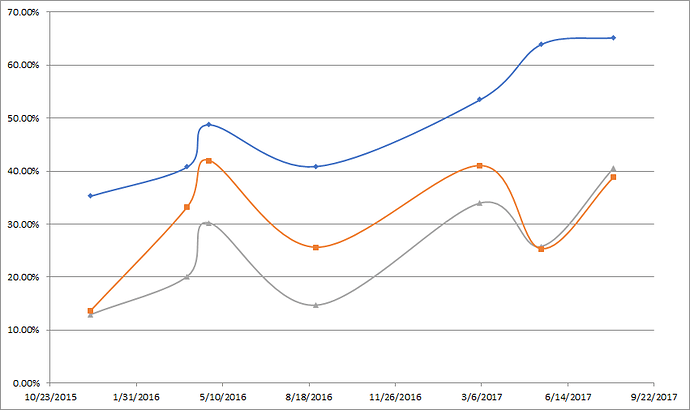
Well, Kurtis, you were probably correct. Here are the same results with the addition of an extra column giving the out-of-sample alpha for the thirty months immediately after the strategy was last updated. In the chart below the results are in orange. There’s some improvement from the first to the third system, but after that there isn’t any, and the correlation between in-sample and out-of-sample drops to 0.47.


Yuval,

Thank you for sharing this.

As you expand on this and look at further data in the future, I would recommend that you consider the problems of spurious correlations in time-series data that is not detrended.

There is NOT a lot of great information available by just Googling this but here is a link that does address this somewhat:Detrending Time Series Data

"This kind of spurious correlation is especially likely to occur with time series data, where both X and Y trend upward over time because of long-run increases in population, income, prices, or other factors. When this happens, X and Y may appear to be closely related to each other when, in fact, both are growing independently of each other."

It would probably require taking a course or reading a textbook for anyone to fully understand this. It is part of a broader discussion of making time series data stationary. Pvdb was kind enough to show me my mistakes in this regard in a post a long time ago. Cyberjo was also helpful in making me understand the problems with data that is not detrended.

This is not something that is immediately obvious to everyone. And I am guessing we have all done this at some time in the past. I think I still fail to consider this potential problem at times, still.

And in fact, this is a problem that the authors make in “All That Glitters is not Gold” that James linked to in a separate thread, I think. This is one reason why the correlation of The Sharpe Ratio is positive in this article while the information ratio correlation is negative, I believe. The information ratio detrends the average returns in the numerator of the Sharpe Ratio calculation, and probably, the Sharpe Ratio regression (correlation) should have never been used in this paper. So some very smart people fail to consider this problem even in their publications, it apprears.

Summarized: for stock market data that has an upward trend we should be dealing with excess returns only for correlations. Preferably excess returns compared to the universe, but a highly correlated benchmark may suffice.

Anything else can be misleading or just plain wrong.

Not all members can afford to make that mistake with their money. Not everyone can afford to chase a spurious correlation for years until they find that a port just does not work for reasons they do not understand. Ultimately, I guess, it is a members choice as to whether they want to use excess returns (detrended data) for their correlations, or not. Or whether to make an effort to determine when this may cause a problem.

But IMHO, P123 should make an effort to take this into consideration in its product development.

Members are quick to criticize statistics in this forum. Some have even criticized the normality assumption (or central limit theorem) and the standard deviation used to calculate the correlation coefficient.

Fine. But then it logically follows that we should be even quicker to criticize bad statistics. There should not be a lot of debate about this. Especially from people who claim not like statistics in the first place.

Thank you.

-Jim
Is this still giving the same surprising result?

Ths is interesting.

Can ask you if the universe, that pass the rules shrunk significantlz with each strategy improvement?

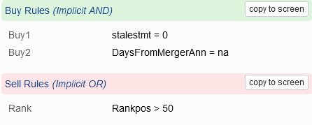
I reran this. I used the Easy to Trade US universe, variable slippage, 20 positions, Russell 2000 as the benchmark, and the buy and sell rules below:
image
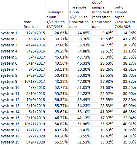
Here are the results:
image

The correlation between in-sample and out-of-sample returns is between 0.47 and 0.58. On average, out-of-sample alpha is about 63% of in-sample alpha.

No, it expanded.

This would appear to demonstrate that the larger the in-sample alpha, the larger the out-of-sample alpha will be. But it says absolutely nothing about the methods used to arrive at the in-sample alpha. If those are not good methods, then the out-of-sample alpha will be bad. I’m not saying my methods are great, but I don’t know if there are any lessons to be learned from such graphs.

The OOS results will be a combination of Alpha and data memorization. Those people who choose poor factors and poor process will get mostly data memorization with little alpha or no alpha.

The real danger is believing that the In Sample results represents some sort of performance that is achievable in the future. It doesn’t. The best you can get is a little advantage in the markets.

Too many factors, too many internal nodes (if a neural net), and all that will happen is the in-sample dataset is memorized. The results look great but you won’t get anything useful out of it.

It is process and expectations that are harmful. Optimization in itself is not harmful.

1 Like

Would you consider someone with total memory recall to be extremely intelligent? Just because he can recite the past doesn’t mean he can intelligently foresee the future. The same goes for system optimization. If you provide too many input factors and don’t optimize properly then you can have a system that accurately predicts the in-sample data series but has no ability to predict the future.

I’m not sure what your issue is. You can never fully eliminate memorization, you can only be aware of it and attempt to minimize it. By doing so, you don’t drown out the predictive power which is relatively small. Does that make sense?