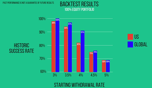
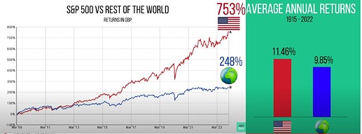
Is average return all that matter? Should you just buy the SP500?

[marco]

Really interesting and good explanation of why annual return is not all you should look at, especially for retirement. I really enjoyed this video and he does a great job with the charts.

What does it mean for P123? That perhaps adding European data was a smart decision! And that we need to focus on other things instead of just great backtested returns. And produce tools that put more emphasis on stability, rather than just average returns (we started doing this a bit with our new rank performance, and AI factor). Lastly we're starting a Risk Model project to help reduce volatility.

Hope you enjoy.

Don't Invest in the S&P 500. Especially if you're retired. (108-year backtest results)

Some screenshots...

What would you choose?

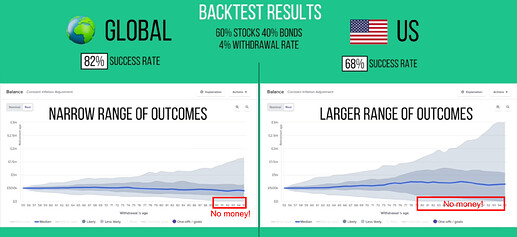
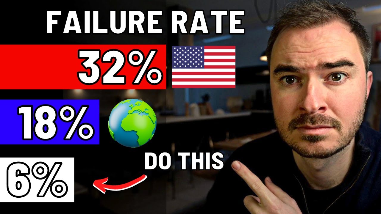
The problem is that when you combine it with an annual withdrawals the SP500 has a much higher change of failure at the 4% withdrawal rate. In other words you'll end up with no money (82% success rate vs 91%)

The problem is volatility of course. If you are lucky in the beginning of retirement, and hit some very good returns with the SP500, you will end up with a lot more money at the end (which you can't take with you). Conversely if you have a string of bad years at the beginning you could run out of money.

Neither is good if your main goal is to enjoy retirement (spend more money every year) with good changes of success.

[mv388158]

I'm over simplifying this but there was a retirement podcast on Resolve Riffs that explored the retirement question:

ReSolve Riffs on "Everything You Need To Know About Saving For Retirement"...

The basics are you need a guaranteed income (Annuity) and stocks. When there is a recession you withdraw from the Annuity and when times are good you withdraw from stocks. One of the trends I am seeing every Robo Advisor is adding some form of private lending. Private lending has exploded over the last 10 years. My friends hedge fund has done 7-8% for 14 years running. There is zero volatility. I just sit back and enjoy the returns. That does not mean zero risk. They are 2 very different animals.

Cheers,
MV

[yuvaltaylor]

@marco

why annual return is not all you should look at, especially for retirement.

I like to look at median annual or quarterly return rather than CAGR for portfolios that I'm planning to withdraw from frequently.

[Jrinne]

You will have to get many members to think differently.

I wanted to code a Monte Carlo Simulation (or Bootstrap Simulation) of a stock strategy using the top bucket of a rank performance test which is about 20 stocks. As you know it is possible to add slippage to a rank performance test. So easy to do for a start right? Just download the rank performance test with slippage onto your desktop and run the code (that reads the csv file from your desktop).

I mindlessly picked a rank performance test I have been looking at recently. I had a nice result for a 4% withdrawal rate for 30 years I think (100% success rate and living well):

Marco, you will have to get members to not believe their sims are necessarily good predictors of future returns is my point. For those who DO BELIEVE their sim results will continue into the future, it won't have much value as their success rates will always be 100%.

Code for those who have a rank performance test they believe is realistic (for Macs with a csv file saved to the desktop). This code could be modified for downloads of book returns:

import pandas as pd
import numpy as np
import matplotlib.pyplot as plt
from scipy import stats

# File path - adjust this to match your file location
file_path = "/Users/yourusername/Desktop/portfolio_returns.csv"

# Read the CSV file
df = pd.read_csv(file_path)

# Assuming the returns are in a column named 'Returns' and are in percent
returns = df['Returns'].values / 100  # Convert percent to decimal

# Simulation parameters
initial_balance = 1000000  # $1 million initial portfolio
retirement_years = [20, 30, 40]  # Different retirement durations to simulate
num_simulations = 10000
annual_withdrawal_rate = 0.04  # 4% annual withdrawal rate

def simulate_portfolio(initial_balance, years, returns, annual_withdrawal_rate):
    """Simulate portfolio value over specified years using weekly returns and withdrawals."""
    num_weeks = int(years * 52)  # Convert years to weeks
    weekly_withdrawal = (initial_balance * annual_withdrawal_rate) / 52
    
    simulated_returns = np.random.choice(returns, size=num_weeks, replace=True)
    portfolio_values = [initial_balance]
    
    for week_return in simulated_returns:
        new_value = portfolio_values[-1] * (1 + week_return) - weekly_withdrawal
        if new_value <= 0:
            portfolio_values.append(0)
            break
        portfolio_values.append(new_value)
    
    # If the simulation ended early, pad with zeros
    portfolio_values += [0] * (num_weeks - len(portfolio_values) + 1)
    return np.array(portfolio_values)

def run_monte_carlo(initial_balance, years, returns, annual_withdrawal_rate, num_simulations=10000):
    """Run Monte Carlo simulation for specified parameters."""
    final_values = []
    for _ in range(num_simulations):
        portfolio_values = simulate_portfolio(initial_balance, years, returns, annual_withdrawal_rate)
        final_values.append(portfolio_values[-1])
    return final_values

def calculate_confidence_interval(data, confidence=0.95):
    """Calculate confidence interval for given data."""
    mean = np.mean(data)
    sem = stats.sem(data)
    return stats.t.interval(confidence, len(data)-1, loc=mean, scale=sem)

# Run simulations and plot results
plt.figure(figsize=(12, 8))

for years in retirement_years:
    final_values = run_monte_carlo(initial_balance, years, returns, annual_withdrawal_rate, num_simulations)
    
    # Calculate confidence interval
    ci = calculate_confidence_interval(final_values)
    
    # Plot histogram
    plt.hist(final_values, bins=50, alpha=0.5, label=f'{years} years')
    
    # Print results
    print(f"\nResults for {years} years of retirement:")
    print(f"Mean final value: ${np.mean(final_values):,.2f}")
    print(f"Median final value: ${np.median(final_values):,.2f}")
    print(f"95% Confidence Interval: (${ci[0]:,.2f}, ${ci[1]:,.2f})")
    
    # Calculate success rate (portfolio not depleted)
    success_rate = (np.array(final_values) > 0).mean()
    print(f"Success rate: {success_rate:.2%}")

    # Calculate real annual return equivalent (accounting for withdrawals)
    total_withdrawals = initial_balance * annual_withdrawal_rate * years
    ending_balance = np.median(final_values)
    real_annual_return = ((ending_balance + total_withdrawals) / initial_balance) ** (1/years) - 1
    print(f"Median real annual return equivalent: {real_annual_return:.2%}")

plt.title(f'Monte Carlo Simulation of Retirement Portfolio\n(Weekly Returns, {annual_withdrawal_rate:.1%} Annual Withdrawal)')
plt.xlabel('Portfolio Value at End of Retirement')
plt.ylabel('Frequency')
plt.legend()
plt.grid(True, alpha=0.3)

# Save the plot as a PNG file on the desktop
plt.savefig('/Users/yourusername/Desktop/retirement_simulation_with_withdrawals.png')
plt.close()

print("\nThe plot has been saved as 'retirement_simulation_with_withdrawals.png' on your desktop.")

[ZGWZ]

@mv388158

My friends hedge fund has done 7-8% for 14 years running. There is zero volatility.

I don't think this is a regular hedge fund, but a straight up Ponzi scheme.

Madoff investment scandal

[InmanRoshi]

FWIW, one thing I've done with one of my Live Portfolios that I withdraw from regularly is systematically change my cash positioning in the portfolio based on perceived market risk. I suppose this could be categorized as Market Timing, but this is not an attempt to maximize Alpha .. or even Sharpe, honestly ... just a way to always have sleep at night cash on hand to ride out a prolonged multi year bear and stay invested without totally liquidating my model.

I created a series of functions that are Red Flags with an eval statement that toggles them to 0 or 1 based on criteria. Simple examples are $UnemploymentRate = 1 if the Unemployment rate goes up. $SMA = 1 if the trend of the SPY falls under its 200 day sma. $FutureEarnings =1 based on the #SPEPSCY simple moving average found in the public P123 screen, etc. I have about 9 or so of these.

Then create a $CashPosition function that aggregates them together
$CashPosition = $UnemploymentRate + $SMA + $FutureEarnings

Now in the Buy and Sell rule of a Live Portfolio I have a Change the CashPct of the port depending on the $CashPosition aggregated, and the cash positioning drifts from ~10% to ~30% accordingly.

Buy Rule

Eval($CashPosition=0,CashPct>9,Eval($CashPosition=1,CashPct>14,Eval($CashPosition=2,CashPct>19,Eval($CashPosition=3,CashPct>24,CashPct<30))))

The opposite on Sell Rule

Eval($CashPosition=0,CashPct<9,Eval($CashPosition=1,CashPct<14,Eval($CashPosition=2,CashPct<19,Eval($CashPosition=3,CashPct<24, CashPct<30))))

On rebalance, it will adjust the buy and sell recommendations to fit inside the CashPct parameters. It will liquidate my lowest rank stocked if I don't have the specified percentage of cash on hand in the portfolio. It will add more positions from the cash if the aggregate flag starts to get smaller.

I hold the cash positioning in $SGOV or $BOXX to draw a few percentage points of interest.

Note, this is only in one account where I regularly pull money out of. I'm really not a believer in Market Timing in general, and don't incorporate this concept in most of my models .. particularly not in my long term horizon retirement accounts. I just look at it like I'm building a castle defense around my wealth, and this is series of moats that has to get cross over before a bear market can get to my stash.

[InmanRoshi]

I agree with Marco's point about how it was a good idea to add European Stocks. My longest term investment horizon accounts incorporate US and European stocks, even if it's been somewhat of a short term drag recently. I also think adding Asia Pacific markets would be a fantastic addition to P123. If we've past post ww2 peak globalization and we're going to move into more of a multi-polar global economy, regional diversification is going to be imperative to avoid catastrophic over concentration risk. Particularly for US investors who are starting at very high historic valuations. The Forward PE for the SPY is now around ~22, around a 20% premium to the PE of the previous 10 years of 18. I lot of forward earnings growth is already baked into the price. If actual earnings fall short of expectations it's not going to be pretty. Any reversion back to a multiple contraction regime is going to probably be long, painful and multi year (ala 2000-2003) imo.