Quantifying Backtest Overfitting in Alternative Beta Strategies / Alternative Risk Premia Is the Selection Process Importan

Georg,

I have just send these two academic papers to Jim via email and thought that you should have them too. (as well as anyone who is interested to know more about overfitting backtested via live returns).

Recently, I have become concern about the issues of overfitting again and found these two papers (both rather difficult to obtain). Both papers suggests that it is very easy to overfit and according to their research, we need to take at least a 75% haircut on sharpe/sortino and backtested return to get close to return with Live data.

Regards
James


Quantifying Backtest Overfitting in Alternative Beta Strategies.pdf (1.01 MB)


Alternative Risk Premia Is the Selection Process Important.pdf (1.67 MB)

James, thank you for those papers.
How are we going to ensure that strategies backtested on the P123 platform are not overfitted?

Best, Georg

Georg,

I think I would not have any better answer than you have on this. I think you have offered one possible solution for some situations: piggybacking.

If one can start with something that is known to work out-of-sample maybe the noise we add with our overfitting will not be so harmful. Maybe we will continue to outperform the benchmark out-of-sample despite our overfitting.

Obviously not a complete discussion on the topic. But I think this is a good idea.

Jim

Georg,

That is a good question.

According to what I learnt from several different papers one way is to do cross validation, ie use the past 15-5 years to perform the backtest (train) and then use the most recent 5 years to validate if it is working. Another way is to keep the backtested strategies as simple and straight forward as possible (the more complex it is, the highly the chance of overfitting.)

There are other more complex methods to test for overfitting, I will leave that for Jim (the expert) to comment.

Regards
James

James,

As you know you have used piggybacking and have made some money doing this–maybe a lot of money. You developed most of these ideas on your own, I think. Certainly not with any significant help from me. We have discussed a few ideas together but most of the ideas were yours and you implemented at least some of your own ideas for your trading.

I will let you share any details. I am not sure I know the details on how your strategies are doing recently or how you may have modified them based on your experiences with these strategies.

Jim

Georg,

Since Jim is being humble (again), I will try my best to show how to detect overfitting with more complex methods that I have read from some research papers. For more information, you can look up these by googling them up or ask Jim if he wants to explain them further.

There are mainly two broad approaches to deal with multiple hypothesis testing, namely family-wise error rate (FWER) and the false discovery rate (FDR).

FWER

The strictest multiple hypothesis test is to try and avoid any false rejections. This translates to control the FWER, which is defined as the probability of rejecting even one of the true null hypothesis and therefore the FWER measures the probability of even one false discovery. There are two main FWER tests.

Bonferroni Method

The Bonferroni method is a single-step procedure since all p-values are compared to a single critical value. This critical p-value is =M, where is the critical value chosen and M is number of rules examined. For a large number of rules, this adjustment leads to an extremely small critical p- value which makes it very conservative and leads to a loss of power. The lack of power is due to the
fact that is implicitly treats all test statistics as independent and therefore ignores cross-correlation that is bound to be present in the technical trading rules employed in this study.

Holm Method

The Holm method is a stepwise adjustment that that rejects the null hypothesis of no out- performing rules if pi =(M 􀀀 i + 1) for i = 1; :::m. Compared to the Bonferroni method, the Holm method becomes less strict for large p-values. Thus the Holm method typically rejects more hypotheses and is more power than the Bonferroni method. However, it also does not take into
account the dependence structure of the individual p-values and is very conservative.

FDR

Rather than controlling for the number of false rejections, we can control for the proportion of false rejections of the False Discovery Proportion (FDP). FDR measures and controls the expected FDP among all discoveries where a multiple hypothesis testing method is said to control FDR at level if FDR E(FDP) , where the level is user-defined.

BH Method
One of the earliest FDR controlling methods is by Benjamini and Hochberg (1995) and is a stepwise procedure that, assuming all individual p-values are ordered from smallest to largest and defining:

Where we reject all hypothesis H1;H2; :::;Hj . This is a step-up method that starts with examining the least significant hypothesis and moves up to more significant test statistics.

BY Method

Although Benjamini and Hochberg (1995) show that their method methods FDR if the p- values are mutually independent, Benjamini and Yekutieli (2001) show that a more general control of FDR under a more arbitrary dependence structure of p-values can be achieved by replacing the definition of j. However this method is less powerful than the BH method and is still very conservative. We employ these four multiple hypothesis testing procedures on the individual p-values of each trading rule. Consistent with Bajgrowicz and Scaillet (2012), to acquire individual p-values, we follow the re-sampling procedure of Sullivan et al. (1999). We employ the stationary bootstrap method of Politis and Romano (1994) to resample the returns of each strategy, where the corresponding test statistic for each bootstrap series of returns is calculated by comparing the original p-value with the bootstrapped p-values.

I am not being humble. I am actually doing some piggybacking which I learned from Georg and James.

I can tell you what I would like to try if I could.

Investars has classification data (or one might prefer to call them ordinal, nominal or dummy variables) from a lot of analysts: Buy, Hold, Sell. There may be less problems with overfitting with these “classifications” because there are no problems with outliers and because there are so many stocks in each “classification”. I get that classification generally refers to the target variable, so I would like to use Investars buy, hold and sell data from analysts to classify the returns.

I would like to run a random forest classifier on this data.

No reply back on whether Investars is willing to partner with me on that. Meaning, I am not sure what data to try it on.

In the mean time, I give credit to James and Georg for what I am able to actively pursue with stocks. I am doing a few things with ETFs. Some of them were developed with James’ help.

Overfitting is a difficult topic. The above is just an idea.

Jim

For those who don’t want to download and read the whole paper.

Here are the summaries by Alpha Architect & CXO Advisory for the paper Quantifying Backtest Overfitting in Alternative Beta Strategies :

https://alphaarchitect.com/2016/05/09/beware-of-backtest-overfitting/

https://alphaarchitect.com/2018/08/20/looking-at-alternatives-avoid-complexity-and-magical-backtests/

https://www.cxoadvisory.com/big-ideas/live-performance-of-alternative-beta-products/

Regards
James

So there is a general answer to this question:

  1. Occam’s Razor

  2. Where possible: use something that has worked out-of-sample and is not cherry-picked.

Not that this as easy as it may sound or that there might not be many ways to try to implement this. And I certainly do not want to start an endless debate on the specifics of how this might be achieved beyond what I have already said: Georg and James have a good idea.

I’m afraid I don’t understand how anyone could expect out-of-sample data, in any field, to be as clean and beautiful as backtested and optimized data. Backtesting with a view to optimization–and it’s very hard to create a backtested strategy without some optimization, as even a simple acceptance or rejection of a hypothesis will lead to some degree of optimization–is not illegitimate or useless or non-predictive. But one has to be prepared for out-of-sample performance to lag optimized performance, because it almost invariably will. The authors write, “we will examine the realized returns and risks of the strategies and, specifically, the persistence of risk-adjusted returns after the “live” date—that is, when the strategies are launched in the market with a final and published investment algorithm,” because this “allows us to quantify the possible biases in strategy construction.” On the contrary, it’s just an inspection of the obvious.

As for Georg’s question, statisticians have been studying this and have lots of answers along the lines that James outlines. But I think a non-statistical approach also has some value here.

A strategy is more likely to be overfitted if it involves a relatively small sample. For example, let’s take a market-timing strategy that gets in and out of the market over the last twenty years. Even if it does so twenty times, that’s still an incredibly small number of transactions on a very small amount of data (the data consisting of the daily returns of an index, or several closely correlated indexes). On the other hand, a market-timing strategy that is run over a hundred years on the relatively uncorrelated indexes of fifteen or more different countries and economies, including such outliers as Japan, India, Brazil, and Russia, would probably have more persistence. Or let’s take a piggybacking strategy that chooses ten stocks out of a universe of fifty stocks held by an index-based ETF. Again, the maximum number of transactions one can test is going to be very small. A strategy, on the other hand, that chooses 100 or 200 stocks out of the thousands available in All Fundamentals, and does so by first splitting up that universe into random subgroups–and maybe the time period into randomized subgroups–and uses a period of more than ten years–will probably have more persistence out of sample simply because the sample size is so large, as is the number of transactions tested; in addition, one can see the way the test results vary from sample to sample. Lastly, all backtesting should be take care to discount outliers, which can be not just securities but also short time periods. It is not hard to statistically identify time periods that are so unusual or extreme that their inclusion in a backtest will make the results less predictive, and to exclude those from the backtest. For example, I have seen many backtests in which all the outperformance is concentrated in a very specific time period. By excluding that time period and rerunning the backtest, you can guard to some degree against overfitting.

I’m sure there are statistical measures that codify all this much better than I have done, but this is what makes common sense to me–as someone who has run tons of backtests and has gotten out-of-sample returns that are impressive, even if they fall significantly short of the backtested returns, which is what I’d expect.

Lastly, even if a strategy is not overfitted, and even if your backtests are impressive and impervious to outliers, there’s still a damn good chance your out-of-sample returns are going to be horrible. What you’re trying to do with proper backtesting is to minimize that chance.

Yuval,

Excellent post and I basically agree with almost everything.

But you miss the point on SOME piggybacking strategies. Sometimes when you piggyback you are piggybacking on somthing that has already proven itself out-of-sample. Not always but it is at least possible. And to the extent that it can be done it could be a good idea.

An extreme example would be: it would have been nice to be able to piggyback on Peter Lynch’s Magellan Fund when he was around.

Of course, one could argue whether the Magellan Fund is a realistic example of what could be done by piggybacking an ETF today. And also how timely the information you can get would be for the best performing funds (say hedge funds or George Soros’ funds). These are details one will have to consider when deciding whether to use a piggybacking strategy.

More basically, if I have drawn 20 white balls in a row out of a bag and another has shown about 50% black balls and 50% white balls which bag will I chose to draw from if I am going to bet I will draw a white ball? Statistically, it does not need to made any more difficult than that.

Also you talk about numbers as being a problem with piggybacking but another thread discussed the possibility of piggybacking Zacks Rank one or two stocks. Whether that is ultimately a good strategy, or not, numbers are not a problem here. There are a lot of stocks that have been ranked one or two since 1988 in Zacks out-of-sample data.

Certainly there is a little more data for some piggybacking candidates than any of the Designer Models that P123 makes available. But data is not everything as you imply in your post. There are some good Designer Models that I would be very comfortable with, but I would prefer to piggyback on someone like Peter Lynch (where possible).

It can be rational in some situations (not all by any means).

Agreed. Regression toward the mean would cause this if nothing else. Like I said, I agree with almost everything.

BTW, I was not making a feature request. I’ll use InList if I want to do this and be happy that P123 makes InList available.

Jim

Yuval,

While I generally agree with what you say about using common sense versus mathematical proof and while I am not a mathematician, you should take a look at this new article from Marcos LĂłpez de Prado (a leading figure in machine learning and AI for investment) that we should really control the number of trials on backtesting in order to prevent finding false investment strategies.

https://twitter.com/lopezdeprado/status/1456938378423844866

The full article is here :

https://www.tandfonline.com/doi/full/10.1080/00029890.2021.1965068

Regards
James

De Prado makes some great points in his paper I think. There are a lot of good ways to prevent overfitting.

Sometimes the methods have names in textbooks. Some of those textbooks have written by de Prado. Some ideas we see at P123 are developed independently. Some of these seem somewhat similar to what de Prado has written but are given different names here at P123. As a general rule most of what we see at P123 makes sense if given a chance. Some ideas are petty labor intensive, however.

Is P123 getting Russian data?

Anyway, Yuval can expand on his ideas without my help. Marc too. But I think it is fair to say that Marc did not do a lot of overfitting and I think he might not mind me making that observation.

Jim

Lopez de Prado and Bailey look only at one aspect of backtesting: the number of trials. They do not examine the number of samples tested or the size of the population being tested. Taken together, I would argue that those two variables are more significant than the number of trials in determining overfitting. For example, if you were to attempt to get the right dosage of a drug by doing repeated tests on the same twenty people, your results would be ridiculous. That is parallel to the approach the authors warn against. But if you were to take a thousand people and give them different doses, your results might be less precise but would be far sounder. Fewer backtests, larger sample. (There may be a parallel here to piggybacking, but I won’t go into that.)

There are two dangers in backtesting: overfitting and undertesting. We have to find the right balance. Which is worse: a strategy that is overfitted but takes into account a myriad of different possibilities, or a strategy that is undertested and is therefore more susceptible to unforeseen factors? To use the above example, before a drug goes to market it is imperative to get the dosage correct. Undertesting may result in overdoses. Overfitting is a problem with small sample sizes. But given a large enough sample (say, a thousand people), running twenty tests is probably better at determining the optimal dosage than running two.

Yuval,

Despite my background in Finance and Applied Statistics and studied at a post graduate level, I don’t think I am smart enough to debate/argue with Marcos López de Prado that they do not examine the number of samples tested or the size of the population being tested in his academic work/textbook after it has been peer-reviewed and published on the The American Mathematical Monthly.

Regards
James

Duckruck,

It has been a while since my last post in P123, I saw your message and want to give you a reply. Here is a brief update for the haircut on Sharpe recommended based on a recent research.

Tab. 1 Comparison of Sharpe Ratios of backtested strategies Sharpe Ratio (of)
average median
in-sample results 1.574 1.180
out-of-sample results 1.049 0.662
Δ (in-out) -0.525 -0.518
Δ% (in/out) -33.37% -43.90%

Here is the complete document. The link function does not work for this site.

Regards
James

In-Sample vs. Out-Of-Sample Analysis of Trading Strategies

2.June 2023

Science has been in a “replication crisis” for more than a decade. Researchers have discovered, over and over, that lots of findings in fields like psychology, sociology, medicine, and economics don’t hold up when other researchers try to replicate them. There are many interesting questions of philosophy of science, for example: Is the problem just that we test for “statistical significance” — the likelihood that similarly strong results could have occurred by chance — in a nuance-free way? Is it that null results (that is when a study finds no detectable effects) are ignored while positive ones make it into journals? Simply said: many published studies cannot be replicated.

But what does it mean to us, investors and traders? We, here at Quantpedia, try to present you academic research in a digestible form for the person that is not used to going rigorously through myriads of papers written in “academese” and often hard to understand true applicable meaning of it.

So, is there any “edge” in purely academic-developed trading strategies and investment approaches after publishing, or will they perish shortly after becoming public? After some time, we are about to revisit our own concept and test the out-of-sample decay. But this time, we have hard data – our regularly updated database of replicated quant strategies.

Introduction

When an anomaly is discovered and a strategy built around it is shared, it often leads to concerns that the anomaly might be arbitraged away and potentially turning unprofitable in investors’ portfolios. However, investment strategies typically remain profitable after publication, although there is a decrease in profitability. However, the returns do not instantly weaken; a significant part of the return remains even after the strategy becomes widely known. A study conducted by McLean and Pontiff found that portfolio returns were 26% lower out-of-sample and 58% lower during the five years post-publication, indicating that investors are aware of academic publications and learn about mispricing. However, the diminishing of returns happens gradually over time, and even after five years, a remarkable part of an anomaly’s return is preserved. The known anomaly often transforms into a ‘smart beta factor’ and can still be profitably used within a diversified portfolio. It’s also noted that the publication process of academic papers can take one or two years, and during this time, practitioners can extract ideas from working papers to gain an advantage.

A recent paper by Jensen, Kelly & Pedersen: Is There a Replication Crisis in Finance? also discusses the replication of trading strategies described in academic research. The researchers found that over 80% of US equity factors remained significant even after making adjustments for consistent and more implementable factor construction while still preserving the original signal. In addition, the same quality and quantity of behavior were observed across 153 factors in 93 countries, suggesting a high degree of external validity in factor research. That’s really not a bad result …

Not too much disturbing are also findings from Heiko Jacobs and Sebastian Muller in their Anomalies across the globe: Once public, no longer existent? Motivated by McLean and Pontiff (2016) (which we will mention later), they studied the pre- and post-publication return predictability of 231 cross-sectional anomalies in 39 stock markets. Based on more than two million anomaly country months, their result is that the United States is the only country with a reliable post-publication decline in long/short returns. This might provide invaluable insights into the modeling of the “longevity” of strategies performed on these markets and “life expectancy” until strategy/anomaly “dies.”

The last research paper that we would like to mention is that of Falck, Rej, and Thesmar (2021), which examines the hypothesis of ex-ante characteristics empirically predicting the out-of-sample (they define out-of-sample as the post-publication period) drop in risk-adjusted performance of published stock anomalies. Their final conclusion is that every year, the Sharpe decay of newly-published factors increases by around 5% (which is not so much).

Data & Methodology

We have collected all data about strategies from our backtests (the ones you see in the end section of most of the Quantpedia Strategies found in our Screener) that were done in QuantConnect. Next, we diligently get information about when the data from the source papers end (end of data set testing period in the source academic paper). This bases the intersection between out-of-sample and in-sample for our backtests. Next, we divide these data into those two sets and compare and analyze them.

Let’s now show you our selected methodology for this experimental validation of our backtests on one example:

Let’s use our first-ever encyclopedic entry, the evergreen Asset Class Trend-Following strategy, based on Mebane Faber’s paper A Quantitative Approach to Tactical Asset Allocation. End of the backtesting period from paper sets point of intercept between datasets (the year after the hyphen) (on picture highlighted with green):

And this is being that year shown in QUANTCONNECT backtest. Up until the last day of 2008, we consider it in-sample backtest results, onwards from the first trading day of 2009 out-of-sample backtest results.

From all 868 strategies at the moment of analysis (at the beginning of May 2023), we have in-house backtested 671 out of them. Out of those, 417 were maintained and updated on a monthly basis, and those were therefore included in the analysis (and they can also be further used in Quantpedia Pro‘s Portfolio Manager and analytical tools). Further, 62 of them were excluded; we did not have data to get back into the period ending from the paper (we started backtesting from a date later than the end date of the data sample indicated in the paper). This concludes the data preprocessing part. So, we are left with 355 strategies for further analysis.

The main analyzed core interest is the Sharpe Ratio, which we conclude is the most suitable measure to compare in- vs. out-of-sample results in our data sample. Our database covers all main asset classes (equities, bonds, commodities, cryptos). Therefore, it would be meaningless to draw conclusions from annualized return measures when our data sample contains highly volatile crypto strategies and, at the same time, low volatile fixed-income strategies. The Sharpe ratio measure is great in our case because we scale annualized returns by yearly volatility, which helps to analyze risk-adjusted returns.

So, now we have both:

  • in-sample dataset (usually StartDate from QP until the end of Backtest period from source paper),
  • out-of-sample dataset (end of Backtest period from source paper until the end of QP backtest; in case of one-time-off code with limited data, is fixed, in case of recurring and updating code, always dynamic and adjusted to current month);

We calculated CAR p.a. and Volatility p.a., which division gave us Sharpe Ratios for in-sample and out-of-sample for each included strategy.

Results and their Interpretation

Now, let’s move on. As a measure of average, we have chosen the arithmetic mean. The median is the value separating the higher half from the lower half of a data sample and is not skewed by a small proportion of extremely large or small values, providing a better representation of the center. It is the main reason why we include it in our analysis too. The following table depicts the average and median Sharpe Ratios among the in- and out-of-sample data:

Tab. 1 Comparison of Sharpe Ratios of backtested strategies|Sharpe Ratio (of)|average|median|
| — | — | — |
|in-sample results|1.574|1.180|
|out-of-sample results|1.049|0.662|
|Δ (in-out)|-0.525|-0.518|
|Δ% (in/out)|-33.37%|-43.90%|

As per Tab. 1, Sharpe Ratio for out-of-sample results is worse and deteriorated by 33% (on average) or 44% (median strategy). These results are totally in line and consistent with findings in the previously mentioned research papers and previous blog post we wrote about this topic.

Following is the figure depicting the distribution (histogram) of Sharpe Ratios both in- and out-of-sample:
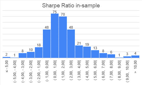
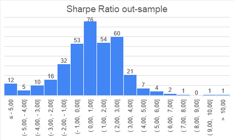
As we can see, the distribution of results follows “quasi-normal distribution”, where you can mainly expect your strategy to have a Sharpe ratio in interval (-1, 3). And it is both for out-of-sample and in-sample results. In-sample results are, of-course, faring a bit better.

Another interesting observation is that both in-sample and out-of-sample results seem to be skewed positively – fat tail on the right side (but the out-of-sample histogram right tail is a little less thick). This is a very interesting finding and speaks in favor of stringent risk management if we employ a portfolio of multiple strategies. It seems strategies seem to deteriorate an out-of-sample, but we have some really strong positive outliers; therefore, it makes sense to cut the risk budget to strategies that do not perform well out-of-sample and let profit runs in those that profit well. Those results may give some validity to the idea of Factor Momentum – it may be a good idea to increase weight for strategies that recently performed well.

But let’s move on. This is the picture showing how all included strategies behaved during the 10-year window, the last 5 years of in-sample, and the first 5 years in out-of-sample:
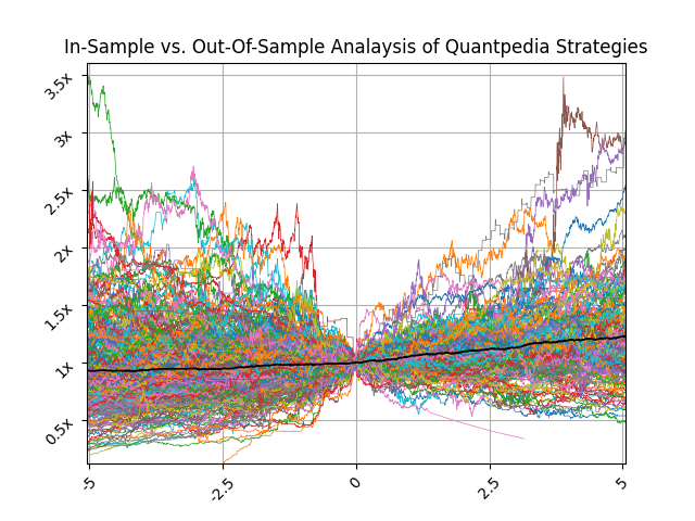
On X-axis, we have an in-sample period (-5 to 0), year zero is the threshold year, and from year 0 to 5 is the performance in the out-of-sample period. Y-axis shows an appreciation of 1 USD during the previously mentioned time. All strategies in year 0 start at 1 USD. The black line depicts the (simple arithmetic) average multiplier of returns when we mix all strategies in an equally-weighted portfolio. Our point here is to show that performed strategies have positive expectancy, but dispersion in performance (in- and also out-of-sample) is really significant.

Assuming we build a portfolio incorporating all backtested strategies weighted equally (black line), we also calculated what would be signal loss in performance after publication. Following our indicated approach, if you start using each strategy on the date when it ends being backtested by paper and weight your portfolio equally, we found that the out-of-sample portfolio would on average yield approximately 4/5 of in sample performance. Once again, individual performance decay among strategies varies a lot.

The performance decay in the portfolio approach is lower than performance decay in individual strategies. The reason for that is the low correlation among strategies (in- and also out-of-sample).

Conclusion

Undoubtedly, Sharpe Ratio s worsen during a lifetime after forming various trading strategies based on beforehand not-know market anomalies. According to our analysis, it is reasonable to expect a Sharpe ratio degradation by 1/3 or by 1/2 against the in-sample period. This should not be, by any means, discouraging, but rather a positive finding that one should embrace and prepare to account for less pleasant sides of investing and trading, considering reported and expected returns and unexpected deviations from them.

Our results are in line with the current academic consensus. As in our previously mentioned blog post from 2020, McLean and Pontiff (2016) find that portfolio returns performing various trading strategies based on a statistically significant sample of different variables and factors covering the representable number of anomalies in total are 26% lower out-of-sample and 58% lower post-publication, which is not far away from our numbers.

What could be the partial solution for the performance decay? Preliminary findings suggest that factor momentum could be the right answer. Fat-tailed financial distributions are known to be good targets to exploit by momentum/trend-following rules. So momentum/trend overlay on a portfolio of strategies can be a good idea. Alternatively, other price-based factor overlays (low volatility, MIX, MAX, etc.) may also be considered, as we reviewed in our series of blog posts in which we investigated Social Trading Multi-Strategy (1, 2, 3, and 4).

Author:
Cyril Dujava, Quant Analyst, Quantpedia

1 Like

Duckruck,

Agreed that a 50% haricut for Sharpe on current DM models is a more conservative level.

The two academic papers (written about 10 years ago) attached at the top of this thread actually recommends a 75% haricut on sharpe/sortino. However, it should be noted that the topic of “overfitting” was less researched 10 years ago and most backtestings done by investment banks and institutions at that time were subject to more serious overfitting.

Regards
James