Thank you again for your very practical feedback.

I had a few questions, and I am also attaching my amateur code that I have started on:

- Over a period of 20 years, how many training periods should it be divided into, and how long should they be in relation to the testing period?
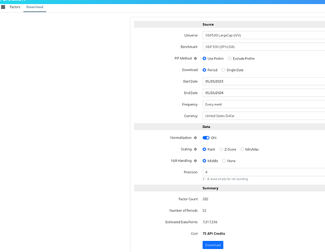
- Is there any problem or consideration I should keep in mind if I test all 282 of my nodes simultaneously?
- If the model is primarily trained to find factors for micro-pg smallcap, do you usually limit the universe to just this, or should I include as many stocks as possible?
*- Are there any other practical considerations that are important to keep in mind when trying to create a machine learning model outside of the solution that p123 provides?*
[size=1]# Install required packages
!pip install pandas scikit-learn xgboost matplotlib seaborn
import pandas as pd
from sklearn.model_selection import train_test_split, KFold, cross_val_score
from sklearn.preprocessing import StandardScaler, LabelEncoder
from sklearn.ensemble import RandomForestClassifier, ExtraTreesClassifier, VotingClassifier
from sklearn.linear_model import RidgeClassifier
from sklearn.svm import SVC
from xgboost import XGBClassifier
from sklearn.metrics import classification_report, confusion_matrix
from sklearn.feature_selection import SelectFromModel
from sklearn.pipeline import Pipeline
import matplotlib.pyplot as plt
import numpy as np
Load the Google Sheets data
sheet_url = "https://docs.google.com/spreadsheets/d/1htu8gJFBZw8nCsn0EGfNqEO3Bgq5WYiT/export?format=xlsx"
data = pd.read_excel(sheet_url)
Display the columns of the dataset
print(data.columns)
Check the time period covered by the data
data['Date'] = pd.to_datetime(data['Date'])
min_date = data['Date'].min()
max_date = data['Date'].max()
print(f"Tidsperioden i datasettet er fra {min_date} til {max_date}.")
Keep a copy of the 'Ticker' column for final display
tickers = data[['Ticker']]
Preprocess the data
Drop columns that are not needed for modeling except 'Ticker'
data = data.drop(columns=['Date', 'P123 ID'])
Handle missing values
data = data.dropna()
Define the target and features
target_column = '1215. Earnings Estimates' # Replace with your actual target column name
X = data.drop(columns=[target_column, 'Ticker']) # Remove 'Ticker' as it is non-numeric
Select only numeric columns
X = X.select_dtypes(include=[np.number])
Feature engineering: add some example features
X['mean'] = X.mean(axis=1)
X['std'] = X.std(axis=1)
X['max'] = X.max(axis=1)
X['min'] = X.min(axis=1)
y = data[target_column]
Convert continuous target to categorical
For example, let's categorize earnings estimates into low, medium, and high
y_binned = pd.qcut(y, q=3, labels=['low', 'medium', 'high'])
Encode target labels with value between 0 and n_classes-1
label_encoder = LabelEncoder()
y_encoded = label_encoder.fit_transform(y_binned)
Split the data into training and testing sets
X_train, X_test, y_train, y_test = train_test_split(X, y_encoded, test_size=0.2, random_state=42)
Create a pipeline with scaling and feature selection
pipeline = Pipeline([
('scaler', StandardScaler()),
('selector', SelectFromModel(ExtraTreesClassifier(random_state=42)))
])
Fit the pipeline on the training data
X_train_transformed = pipeline.fit_transform(X_train, y_train)
X_test_transformed = pipeline.transform(X_test)
Initialize the models
models = {
'Random Forest': RandomForestClassifier(random_state=42),
'Extra Trees': ExtraTreesClassifier(random_state=42),
'Ridge Classifier': RidgeClassifier(),
'XGBoost': XGBClassifier(random_state=42),
'SVM': SVC(probability=True, random_state=42)
}
Train and evaluate each model using cross-validation
kf = KFold(n_splits=5, shuffle=True, random_state=42)
model_performance = {}
for model_name, model in models.items():
print(f"Training {model_name}...")
cv_scores = cross_val_score(model, X_train_transformed, y_train, cv=kf, scoring='f1_weighted')
model_performance[model_name] = {
    'Mean F1 Score': cv_scores.mean(),
    'Standard Deviation': cv_scores.std()
}

print(f"{model_name} Mean F1 Score: {cv_scores.mean()} (+/- {cv_scores.std() * 2})\n")
Print the performance of each model
performance_df = pd.DataFrame(model_performance).T
print("Model Performance Comparison:")
print(performance_df)
Initialize and train Voting Classifier
voting_clf = VotingClassifier(estimators=[
('rf', models['Random Forest']),
('et', models['Extra Trees']),
('xgb', models['XGBoost'])
], voting='soft')
voting_clf.fit(X_train_transformed, y_train)
voting_pred = voting_clf.predict(X_test_transformed)
print("Voting Classifier Report:")
print(classification_report(y_test, voting_pred))
print("Voting Classifier Confusion Matrix:")
print(confusion_matrix(y_test, voting_pred))
Use the pipeline and best model (here we use Voting Classifier) to predict the categories for the entire dataset
X_transformed = pipeline.transform(X)
data['Predicted Category'] = voting_clf.predict(X_transformed)
data['Predicted Category'] = label_encoder.inverse_transform(data['Predicted Category'])
Filter recommended stocks
recommended_stocks = data[data['Predicted Category'] == 'high']
Sort recommended stocks by feature importance and select top 25
top_recommended_stocks = recommended_stocks.head(25).copy()
Include the 'Ticker' column in the final display
top_recommended_stocks['Ticker'] = tickers.loc[top_recommended_stocks.index, 'Ticker']
Add top 10 important features for each stock (only for tree-based models)
if hasattr(voting_clf, 'estimators_'):
best_model = voting_clf.estimators_[np.argmax([model_performance[model_name]['Mean F1 Score'] for model_name in models.keys()])]
important_features = [X.columns[i] for i in np.argsort(best_model.feature_importances_)[::-1][:10]]
else:
important_features = pipeline.named_steps['selector'].get_support(indices=True)[:10]
important_features = [X.columns[i] for i in important_features]
for feature in important_features:
top_recommended_stocks[feature] = data.loc[top_recommended_stocks.index, feature]
Display the table in the notebook (if using Jupyter)
import seaborn as sns
plt.figure(figsize=(15, 8))
sns.set(style="whitegrid")
sns.set_context("notebook")
Format the display of the DataFrame
styled_table = top_recommended_stocks[['Ticker'] + important_features].style.background_gradient(cmap='YlGnBu').set_properties(**{'text-align': 'center'}).set_table_styles([{
'selector': 'th',
'props': [('font-size', '12pt')]
}])
display(styled_table)
[/size]

