backtesting, data-mining, bootstrapping, and Jim O'Shaughnessy

Walter,

Thanks.

Edit: The formula in the image is commonly used. It is the one I have used. I posted the image thinking it was pretty well accepted (before I thoroughly read the paper). As you know the author of the paper is not a big fan of this approximation and I apologize for being overly simple in my post.

Interesting!

-Jim


Thanks Walter and Jim,

Very interesting, indeed.

It is also interesting that the paper didn’t even mention Ito’s lemma (or the Stratonovich integral), whence the canonical convexity adjustment (i.e., one-half the variance) is derived. The convexity adjustment is often seen as a consequence of Jensen’s inequality since when you take the exponential of some linear function, you turn it into one which is convex up. The convexity adjustment is just then really a correction factor, which while not entirely 100% accurate, is often close enough.

Anyhoo, I know this is off topic from the OOS vs in-sample, but it seems to me that if one is that concerned about geometric means, one could more easily calculate those directly. It’s not like there’s a shortage of computing power…

Agreed, it’s a bit off topic but still useful I think.

If my memory is correct, when I first started seriously using p123, a model’s average daily return was bandied about as a quality metric. The higher the ADR, the better. That appears to have fallen out of favor. Perhaps that’s because it didn’t account for the effect of volatility on geometric average return - the metric we really care about.

Walter

LOL. After trying to put the other formulas into excel I think I understand why the simpler formula might be used. I promise I tried, but never could get A4 in the paper to calc properly to match the data in the paper. Math dummies like me will have to settle :wink: Based on the paper it looks like A4 is the best way to adjust the average return in rolling backtests for the comparison of higher volatilities seen like in small caps.

edit: I just got the calc to match! V = StdDev^2. This is useful to me. Thanks wwasilev for the link to the paper!

Walter,

Excellent point! As you know, another name for this is volatility drag. But these formulas also illustrate why there must be some “volatility harvesting” going on in our ports. Using the simplified formula:

Geometric mean = Arithmetic mean - (standard deviation^2)/2

If you assume the return of each of the stocks in a 5 stock model have about the same return (on average) then the arithmetic mean return for all the stock combined in a port is about the same as the return for the individual stock in the port (on average over a long period). But by combining stocks that are not fully correlated the standard deviation for the port is reduced compared to the standard deviation for individual stocks.

So in this equation the 5 stocks combined will have the same arithmetic mean for the returns as an individual stock would but the combined stocks are not 100% correlated and the standard deviation is reduced.

Or put simply, combining the 5 stocks will reduce the standard deviation compared to a single stock and the geometric return will increased in this equation.

I believe this fits the definition of volatility harvesting and it would be hard for it to be the case that we are not doing a little harvesting in our ports. How much volatility harvesting we are actually doing depends on how correlated our stocks are and how volatile the individual stocks are. And as explicit stated in this simplified proof, it does assume the stocks ranked 1 thru 5 have about the same returns and that the assumptions in the derivation of the equation are correct (e.g., lognormality).

-Jim

Jim, I’ve recently been working with screen of screens, and the interplay you mention is something I’ve noticed as I work with those screens.

An example might be:
Lets say I have 3 or 4 models that work decently and I want to take the very best stocks from each. I’m finding usually if I put those 3 or 4 models together in a screen of screens and select only the top ranked stock from each - well, that’s usually not a very good result - I’m guessing because the volatility is so high (almost always is) and this formula shows how the volatility will bring down compound returns. If I take the top 2 stocks from each model, that’s usually better, but still probably not optimal, and again it’s probably not because there’s something wrong with the top 1-2 ranked stocks, but is a follow-on effect of high volatility. What I’m finding is if I combine the top 3 or 4 stocks from each model, however, that’s usually where I see strongest results. With an average of 8-12 stocks the volatility tends to come down enough so that it creates more benefits that more than offset the decision to select lower ranking stocks.

It’s not an intuitive dynamic (to me anyway), but I think it’s something anyone working with models will run into. At first it’s confusing, because I was testing models and wondering why my top ranked stocks in isolation don’t perform so well - so I’d try to exclude them and compare results, but it didn’t help and usually would hurt results. Ultimately, it’s not a problem with the top ranked stocks being abnormal, it’s more that the effects high volatility are difficult to recover from (although thinking this way might provide ideas about how to take advantage of that volatility via timed trades?), and there’s a benefit to lowering volatility even if means picking more lower ranking stocks. Obviously there’s a balance, but it’s not intuitive at all to me - and I come to it after experimenting with many backtests and head-scratchings. :wink: This provides a goof framework for thinking about it.

Michael,

I tend to make more of this than it deserves. Ever since I read about Shannon’s Demon in “Fortune’s Formula” I have been intrigued. I do not think it makes as much of a difference as I once thought. But when we are talking about taking just one stock versus say 5 stocks in a five stock model I think there is an important effect. Also I think some do well with this by shorting stocks in the same industry so that there is a large negative correlation among the stocks—which really reduces the standard deviation and volatility drag substantially. But this is something I cannot do.

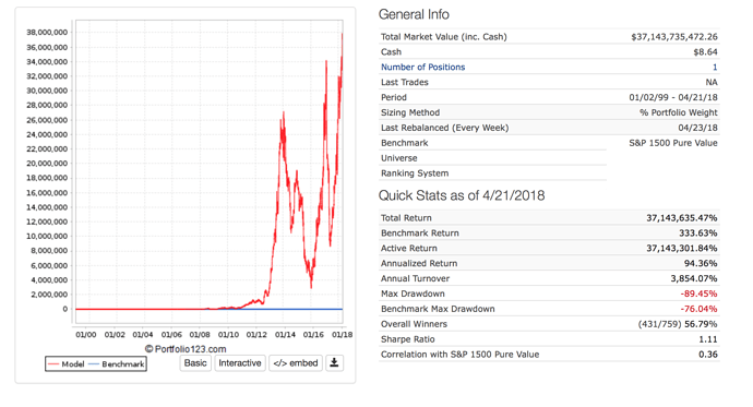
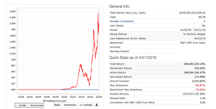
I was playing with some real examples this morning and thought I might share since you have an interest in this. I would like to make a couple of points about these sims before I share them. The main point being these sims ARE TERRIBLE. You can see they have extreme volatility and this is WITH NO SLIPPAGE. But perhaps more importantly they do not perform well out of sample. Needless to say this is not something I use—except, perhaps, to learn about volatility.

  1. Single stock. Weekly return (arithmetic mean): 0.01877, StdDev.: 0.1139, annual returns using calculated geometric mean with simple formula: 89.09%, Annualized return P123: 94.36%.

  2. 2 stocks (always includes the stock in the one stock sim). Weekly return (arithmetic mean): 0.01839, StdDev.: 0.08856, annual returns using calculated geometric mean with simple formula: 114.44%, Annualized return P123: 114.48%

Conclusions. The formula worked well for the 2 stock model but was off a little bit for the one stock model (perhaps close enough for me). There can be a practically significant difference in the volatility drag for one stock versus two stock models. The mean return was higher for a single stock in this example but because of the reduced volatility with 2 stocks the 2 stock model did better.

-Jim


I think this has more to do with diversification than with volatility. Let’s say you have three very high-performing positions. All stocks sometimes go down in price and sometimes go up. The probability that all three stocks will go down at exactly the same time is pretty high. That can seriously damage your portfolio and it will take a lot longer for it to recover. On the other hand, if you add three stocks that aren’t so high performing to the mix, the chances are better that you won’t have that loss.

I’m attaching an Excel file that illustrates this dynamic (ignore the first one, use the second one–the first one has a minor error in it). Columns a, b, and c are stocks that change in price randomly between -15% and +20%. Columns e, f, and g are stocks that change in price randomly between -15% and +18%. Column i is the total portfolio value of holding just columns a, b, and c, and column j is the total portfolio value of all six stocks. You’ll notice at the end of 50 periods, column j is higher than column i about 20 or 30% of the time. If you just look at the individual returns of the stocks, that’s not at all what you’d expect. For example, one run-through had total returns of 76%, 137%, and 124% for the good stocks and 130%, 65%, and 85% for the mediocre stocks. The portfolio of only the good stocks had a total return of 132% while the portfolio of all the stocks had a total return of 135%.

I know there’s a mathematical/statistical principle involved here, but I don’t know what it is or what it’s called . . .


diversification simulation.xlsx (14 KB)


diversification simulation 2.xlsx (13.9 KB)

I find nothing to disagree with.

The mathematical/statistical principles are as above in the previous posts and in your post, I think.

As an aside, I was (still am) a little surprised by the fact that many math courses have no arithmetic in them—just derivation of theorems in english (in the US anyway).

Yuval, IMHO you have posted an excellent example of an existence proof. There exist situations where increased diversity (as defined in your example) or reduced volatility as defined by reduced variance or standard deviation can increase the geometric return. An absolute truth as you have proven in a solid theorem (no matter that the definitions you use may differ).

Perfect IMHO. Well, a little more arithmetic than I like but nearly perfect :wink:

-Jim

Volatility pumping, perhaps?

Yuval, here’s a variation of that idea from where I was toying around with your worksheet.

essentially: sets up a return distribution in deciles, with the a possible return segmented for each decile with the only difference being the best and worst decile having different returns. a,b,c have possible worst/best decile returns of -15% or +15% and e,f,g have worst/best decile returns of -10% or +10%. (I put a 1pp growth bias offset shifting the entire distribution by 1pp per period to the right so the actual range is from -14% to +16%, or -9% to +11%, so average expected monthly return is 1%. That variable in a15 can be changed to 0 to create 0% expected monthly return if desired to isolate the distribution shift).

To isolate the random effects, I’ve set the random seeds that select the return decile to be the same for both a,b,c and e,f,g → so the decile inputs will be randomized, but each group sees the identical random seeds for the return lookups. (column a gets same decile seeds as e, b as f, and c as g)

I’m using Excel 2003, so I hope everything translates OK to whatever version folks are using today.

What I find by pressing F2-Enter to keep recalcing is that a higher percentage of cases result in the lower range of monthly variances producing better geometric returns although the average expected return is the same. I did 100 trials and the scenario with lower ranges on extremes (e,f,g) had better results in 55% of cases - and the version with higher extremes (a,b,c) had better results 45% of the time. My initial gut impression was that the % wins for the lower variance version (efg) was higher than that, so unsure if that trial is representative. I can’t remember how to macro that up for longer trial, so that’ll have to do for now :wink:

Anyhow, wanted to share this in case interested.


diversification+simulation+2_variation.xls (53 KB)

An excerpt from Fortune’s Formula about Shannon’s Demon:

“To make this clear: Imagine you start with $1,000, $500 in stock and $500 in cash. Suppose the stock halves in price the first day. (It’s a really volatile stock.) This gives you a $750 portfolio with $250 in stock and $500 in cash. That is now lopsided in favor of cash. You rebalance by withdrawing $125 from the cash account to buy stock. This leaves you with a newly balanced mix of $375 in stock and $375 cash. Now repeat. The next day, let’s say the stock doubles in price. The $375 in stock jumps to $750. With the $375 in the cash account, you have $1,125. This time you sell some stock, ending up with $562.50 each in stock and cash. Look at what Shannon’s scheme has achieved so far. After a dramatic plunge, the stock’s price is back to where it began. A buy-and-hold investor would have no profit at all. Shannon’s investor has made $125.”

Poundstone, William. Fortune’s Formula: The Untold Story of the Scientific Betting System That Beat the Casinos and Wall Street (pp. 202-203). Farrar, Straus and Giroux. Kindle Edition.

This scheme is highly dependent on the lognormal distribution being an accurate description of the equity’s return which is key to Kelly Criterion, Geometric returns etc. It is the lognormal distribution where halving and doubling are equal moves in opposite directions. But the lognormal distribution has merit.

Anyway, this example is a little extreme but it still blows my mind. Sadly, reality does not yield cash to retail investors—like me—with such an easy or lucrative scheme as this.

-Jim

I would also note that Shannon’s Demon is less pronounced for trending processes, and more pronounced for mean reverting process.

I.e., if you simulate this sort of “diversfiy and rebalance” strategy under an exponential Ornstein-Uhlenbeck process, the returns will increase due to volatility pumping. This has led to speculation as to whether markets require the presence of some momentum in order to prevent free lunches. For what my opinion is worth, I doubt that there a is causal relationship.

Primus,

Wow!. Yep. First part has to be true (and I had not noticed that). The speculation about momentum is new to me. But that is what they do: start with the assumption that there is no free lunch then prove you cannot make money that way (circular). But that does not prove that they are wrong either.

-Jim

I love this. But actually, this is what savvy value investors do every day and always have done: buy more when the price falls and sell some when the price rises.

Yuval,

I am going to admit that I am not sure how much of this I am doing consciously.

But now you see why I wonder how much affect this may be having on my systems: Buy a group of relatively volatile securities and rebalance frequently back towards equal holdings. The rebalancing does not have to be back to exactly equal holdings (as in Shannon’s Demon) for there to be an effect.

Fortunately, this can be quantitated to a large degree using the formulas that Walter provides in his links.

Also, as David (Primus) notes, savvy investors may be doing this except for those investors who put additional money into stocks that are trending. They are in fact doing the opposite.

But there is another very important aspect to David’s compact post that is full of information. NONE OF THIS WORKS IF STOCKS BEHAVE AS A RANDOM WALK (i.e., have a unit root). This is because stocks that behave as a random walk do not regress toward the mean. NOTICE THAT THE STOCK IN SNANNNON’S DEMON EXAMPLE VERY RELIABLY REGRESSED BACK TO THE SAME LEVEL. An example of the EMH advocates assuming that you cannot make money then proving that you cannot make money based on this assumption. Or maybe just a reason to believe that stocks do not behave like a random walk and that markets are not completely efficient.

Anyway, something I will keep looking at.

-Jim

Jim,

Thanks for the mention. I think you’re not giving yourself enough credit for the analysis.

Also, I was hoping you could clarify a few things. You mentioned that:

But then you add:

It appears as though “this scheme” and “this” both refer to Claude Shannon’s demon, but I am not sure really certain I understand the difference. Isn’t GBM just one type of random walk?

Thank you.

//dpa

David,

Let me give you the most simple and accurate answer: I might be wrong about that.

What got me thinking about this is when you said:

Random walks, as you know, do not mean revert.

I guess I wonder if you can expand further on how baldly volatility pumping is affected when the process does not mean revert. I probably jumped to conclusions on this. Maybe it still works as long as it is following a lognormal distribution whether it mean reverts or not? I would be interested in your take on that!

Actually, I am getting pretty sure I was wrong about that but would definitely like to learn more about how mean reverting (or lack of it) affects this!

Thanks!

-Jim

Jim,

Well, now that you mention it, you’ve got me curious as to whether it’ll hold up for a single asset under plain vanilla Brownian motion, mean reverting processes, as well as for multiple risky assets.

I’ve attached something I’ve done in Excel for two uncorrelated Brownian motions (e.g., Wiener processes).

I’ve got some stuff to do in the next few days, but I’ll try come up with some extensions for different types of processes in Mathematica soon.

I’ll keep you posted.

//dpa

EDIT:

There was an error in v2; check out v3.


Shannon's Demon v2.xlsx (53.4 KB)


Shannon's Demon v3.xlsm (52.3 KB)

David,

Thank you for your comments and for the cool spreadsheets!!!

I suspect you had the answer in one of your posts:

I am guessing that whoever authored this idea found that it does work for a geometric random walk and had to add the momentum to get “no free lunch.”

This is kind of how it works with some real investing ideas. We are told that we get some volatility pumping if we split between stocks and bonds. But over long periods the trend in stocks is strong enough that there is no free lunch and we would have received a higher total return if we had put everything into stocks.

My original error is one I tend to make. I imagine a random walk (or the equivalent drunkard’s walk) as the drunk taking off and never coming back. But this is not really true is it? The Gambler’s Ruin theorem proves the drunk, in the random walk, always (eventually) makes it back to the lamp post (at least in the 2-dimensional version of the gambler’s ruin/drunkard’s walk).

But anyway, using the Gambler’s Ruin theorem you can PROBABLY prove there will be profits (volatility pumping) when the stock returns to its previous level or that if there is no net benefit it is because the stock has drift or trend. Of course, it can take a very long time for the drunk to make it back to the lamp post. Perhaps, this is why the authors prefer the quicker moneymaking scheme where the stock in mean reverting. BUT I HAVE A POLICY OF AVOIDING JUMPING TO TOO MANY FALSE CONCLUSION IN LESS THAN 24 HOURS. So I keep an open mind on this.

Anyway I find this interesting and appreciate the opportunity to discuss it. Please continue to post on this as you have more ideas or read more about it!!! And of course, I could still be wrong and would appreciate any corrections as it is preferable to be in error in the posts (and corrected) than to be in error in the market.

-Jim