Evaluating R2G out of sample performance

Today I had a look at the out of sample performance of R2G models. I looked at models that have been launched at least 180 days (around 6 months) ago and are not free. In all, this leaves me with 42 models as of today.

The attached scatter plot of Ann Excess Launch vs Ann Excess Inception shows that there is a very strong correlation between annualized excess return since inception (backtested return) and the annualized excess return since launch (out of sample return). The slope of the red regression line is 0.93, which means that the out of sample excess returns are just a few percent lower than backtested returns. The majority (34 of 42) of the out of sample excess returns are within 20 percentage points of 0.93 * the backtested excess returns. This means that a typical model that has a backtested return of 100%/year has returned between 73% and 113% since launch.

The gain/stock/day of a model is an even more accurate predictor of out of sample performance (in this admittedly limited set of models). In the scatter plot showing Ann Excess Launch vs GSD you can see that the points are closer to the red regression line with fewer outliers.

The only other statistically significant variable is the number of holdings in the model. Using the formula "-44 + 235*(gain/stock/day) + 10log(holdings)" gave the best predictor/explanation of out of sample excess returns I could find. The 235gain/stock/day could also be 252*gain/stock/day (it’s in the confidence interval), so it could be interpreted as gain/stock/year. You can see the predicted out of sample returns versus actual returns in the third scatter plot.

Of course the past year was a bull market, and the fact that models roughly performed similar to their backtests may not necessarily mean they will do so in the future. By using excess returns instead of absolute returns I tried to compensate for the strong performance of the market last year.

Personally I think this proves that R2G models really do outperform the market, and it’s another reason to take gain/stock/day and the number of holdings very seriously when evaluating models.


inception.png


gsd.png


predicted_oos.png

To be clear, you are saying that more holdings are a better predictor of future performance? I don’t quite get the scatter graph.

I raised this issue before: there is a serious flaw in the definition of “market benchmark” for R2G models.

Most R2G models trade micro/small cap stocks while using SP500 as benchmark, and that is why you see OOS excess return.

If you use R2K as benchmark, the result is not encouraging.

If you take into accounts the under-performed R2G models that were deleted, we may need some luck to use R2G to outperform IWM.

If you take into account subscription fee, it may be better just trade IWM or UWM.

However, most free R2G models are really good.

Thanks for showing this. What were the other factors that you tested that turned out to be non-predictive? And could you also show the plot for number of holdings?

Thanks for sharing. It’s nice to see real data in threads and definitely appreciate it. For me, it’s still way too early to know anything. But, please keep posting. Initial results sound promising.

Some questions (if the data is easily available):

  1. What was the average return, range of excess returns and st. dev of excess returns on the models you tested?
  2. If you separate the systems into 2 groups…micro/small cap 750%+ annual turnover vs. all other cap ranges and strat’s - what was the AR by group?
  3. What predictor variables did you test? Did you look at turnover % and trading costs/total port value stats? Number of sub’s (very curious if cost or # of sub’s have any predictive value one way or the other so far)?

Would be great if P123 gave us some ‘R2G analysis’ tools that let us analyze some of the above as the out-of-sample data set grows.

There are several potential issues as hengfu points out:

  1. Inconsistent benchmarks are very problematic. 3 micro-cap systems can have 3 diff. benchmarks. Global systems trading ADR’s and ETF systems often lack any benchmark. This is all issue especially given that the adjustment is excess returns.
  2. Many models launched at potentially great ‘best or top 3 years of the past decade’ times.
    The Russell2000 was up 38% in 2013 vs. 7.7% average over the backtest period (5X a typical year).
    The SP500 was up 32% in 2013 vs. 4.2% average (7.6X average).
    Excess returns helps mitigate this.
  3. No real market DD’s or vol. until the trailing 80 days or so. So…the market timing and hedge components of many systems…a large source of significant risk-adjusted excess returns in backtesting (most likely) have not yet been tested in any real way.
  4. R2G survivorship bias is a potential issue longer term (as hengfu also points out). Were bad models simply deleted?
  5. Length of sample. Very, very short. I’d expect a lot of random noise in 6 months of returns. That’s just what I see when I run tests on ‘Random’ stock selection at various port. sizes from a known universe. Plus, there is very little ability to predict top futures traders returns over a short, go-forward period. But correlations and st. dev’s tend to remain fairly constant.
  6. Sub’s have taxes and model fees to contend with.

Having said all that, sounds like a very good start to R2G. Many systems, and some developers, have had a very good 6-11 months.

My R2G systems have, so far, been disappointing out-of-sample. But…many are low turnover…2 (at least) lack real benchmarks…and none of them are currently over the 180 day threshold you set. So…interesting to see how this all looks in 3-5 years.

Thanks again for sharing.

Best,
Tom

Impressive work!!! If I wasn’t already sold on P123 and a big fan of the R2G authors, I would be now. One quick question and it is a question: are you concerned about just the slope of the regression line or is the y-intercept (-16?) a factor also? Even if it is a factor, I think the returns after launch are still great.

pvdb - is the annual excess compounded or simple? By compounded, I mean if a system has 1% excess gain over a three month lifetime, that doesn’t equate to 4% annual excess, but some higher figure. The stock gain per day is simple. Thus the relationship between annual excess and SGD may be non-linear.

** Edit ** On second thought… SGD compounding is based on turnover. The higher the turnover, the closer to a linear relationship to annual return.

My two cents.
Steve

Some quick improvements from P123 will tremendously help us search for the right R2G:

  1. Add extra columns in R2G Excel download file to show excess return relative to IWM, IWC, QQQ, etc.
    IWC has 45.2% in 2013 v.s. SPY 32.3%. I really want to know the excellent liquid R2G models beating IWC over long term.
  2. Add an extra column in R2G Excel download file to show position sizing.
    This will help us convert and deduct subscription fees from gross excess return.
    $100/month on 5 stocks is significantly costly than $50/month for 50 stocks.
    Right now the excel file only tells number of holdings, which could be significantly different from the actual position sizing.

@plan_trader: well, yes, kind of. I had a closer look, and by itself, more holdings is NOT a predictor of future performance. But when you use it together with G/S/D it does improve the prediction of future performance significantly. I use the word ‘significantly’ here in the statistical sense, not in the sense that the prediction is a whole lot better.

To be more precise, I used LOG(holdings), which is the natural logarithm of the number of holdings. For 5 holdings, this value is 1.6, for 10 holdings it’s 2.3, for 20 holdings it’s 3. The reason I used the logarithm is that I would expect that going from 5 to 10 holdings adds relatively more ‘robustness’ than going from 100 to 105 holdings for example.

The regression found a coefficient of 10 for LOG(holdings). The way to interpret this is that going from 5 to 10 holdings increases LOG(holdings) from 1.6 to 2.3, and this number should be multiplied by 10 to see the effect on the nnual excess return since launch in percentage points. So for two models with the same G/S/D, but one has 5 holdings and the other has 10, the difference in annual excess return since launch would be estimated to be 10 * (2.3 - 1.6) = 7 percentage points. The difference between 10 and 20 holdings would be 10 * (3 - 2.3) = 7%. So doubling the number of holdings adds 7 percentage points.

However, the confidence interval for LOG(holdings) is approx 2.5 to 17.3, which is pretty large. That means that, statistically, this coefficient of 10 is pretty uncertain. It could be anywhere from 2.5 to 17.3. That means that the impact on return of doubling the number of holdings is anywhere between 2.5 * (2.3 - 1.6) = 1.75 to 17.3 * (2.3 - 1.6) = 12 percentage points. So the statistics are saying it’s kind of relevant, but the exact impact on returns is not very certain.

@hengfu: I also think many models do not have the right benchmark. I did not try to correct for this. If you want to take a more ‘pessimistic’ view on excess returns, I think you can just subtract another 13% from the Ann Excess Launch numbers. The correlation would still be the same though.

Whether a model is worth the monthly fee is an entirely different discussion, and depends to a large extent on the amount of money a sub wants to put into a model (keeping liquidity constraints in mind of course). The question of which model(s) to invest in is indeed more complicated.

@MisterChang: I basically tested all the factors that are in the Excel spreadsheet that you can download from the page with the list of all R2G models. Specifically, the other factors I looked at are: AVG_RET_LOSERS, AVG_RET_WINNERS, COST, DRAWDOWN, LIQUIDITY, SUBS, TURNOVER, VIEWS, WINNERS, YIELD. I also calculated the average return (both winners and losers) and the number of trades per year.

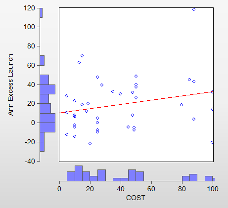
In particular, the cost (monthly fee) has no correlation with out of sample excess returns. This was a bit of a surprise to me. See the attached scatter plot. The red line shows a (slightly) increasing return for higher cost models, but this is not statistically significant. (Btw, I excluded one model with a fee of $250 in this plot).

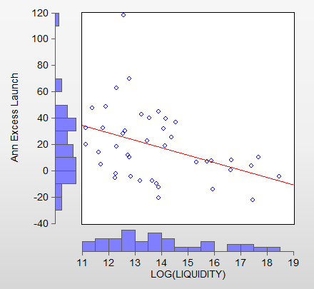
There is definitely a relationship with liquidity, but it’s not a simple linear or LOG(linear) relationship. Lower liquidity models definitely have higher returns, but the scatter plot shows that the points are pretty widely dispersed around the regression line, so statistically speaking it’s not very certain what the exact relation is.

@Tomyani:

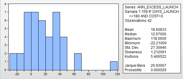
  1. see attached histogram with statistics
  2. If I use “liquidity < $1MM and turnover > 750” then the sample only contains 11 models (out of 42). This is really too small to draw any conclusions I think.
  3. I did not look into trading costs, but I did look at turnover and number of subs. By themselves, they had no predictive value. But turnover is the difference between simple AR and G/S/D, and it’s the reason that G/S/D works better than just AR. The number of subs would only make sense if you include liquidity somehow I think, but I didn’t look into that. There must be better ways to find impact on slippage (which is what I’d be trying to find by looking at subs).

Regarding your other points, all of which I agree with:
3) yes, market timing and hedging have been (barely) triggered, so this could be a very important reason why the correlation I have shown would not hold up in the future. Actually, I was thinking that if R2G models all have very high beta, than the results I got are what you’d expect, but in a down market the models would incur very large losses. Especially if the market timing / hedging does not work out of sample.
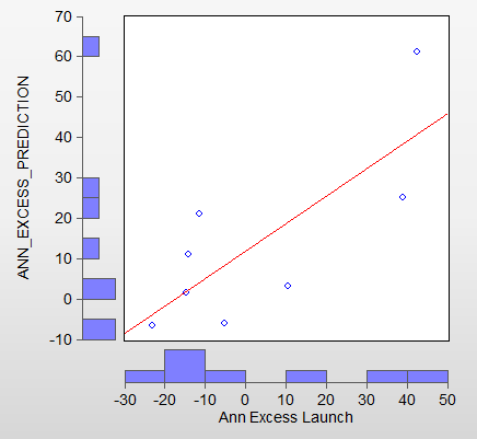
5) The correlation gradually breaks down when I include models with more recent launch dates. There is basically no correlation whatsoever for models that have been launched in the past few months. I don’t know whether that is due to random short term fluctuations or the fact that the market is at the same level as it was a few months ago (ie correlation only holds in bull markets because of high beta).

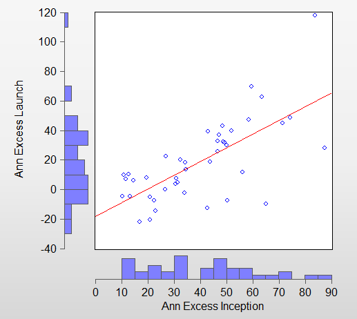
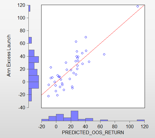
@Jrinne: the slope is near perfect, meaning it’s almost a one-on-one correlation between in-sample and out-of-sample performance. I think the intercept of -44 in my -44 + 234GSD + 10LOG(holdings) can be explained as follows. One part of the intercept corrects for the return of the market (roughly 30% or so). The GSD is a measure of absolute performance, while I’m regressing on the excess returns. The difference between absolute and excess return last year was around 30%. The other part is correcting for the LOG(holdings) component. A model needs to have at least 5 holdings, so every model will always score 10 * LOG(5) = 10 * 1.6 = 16 percentage points “for free”. This is corrected by the intercept. Adding 30 and 16 gives 46, which almost exactly explains the -44 intercept.

@Steve: I used the annualized numbers that P123 reports. Because I only used models that were live for at least half a year, I don’t think this a very big issue, if at all.

Thanks for your insightful comments!


cost.png


ann_excess_return_stats.png


log_liquidity.png

I was referring to the above part of your post. More accurate to say: y = 0.93 * the backtested excess returns - 16. This means that a typical model that has a backtested return of 100%/year has returned between 57% and 97% since since launch.

Your first graph clearly has a y-intercept below 0. Y = mx + b(y-intercept).

I actually think this is excellent (both the results and your statistics). The decline in out-of-sample results is real, expected and mild as your statistics show.

Hi pdvb,

Thanks for your work. What software do you use for your scatter plots ?

Yes! Thank you for doing this study pvdb.

“I used the annualized numbers that P123 reports. Because I only used models that were live for at least half a year, I don’t think this a very big issue, if at all.”

I wasn’t really making myself clear. The annualized excess returns are not a big issue but I’m more concerned about stock turnover. For example, looking at all systems in the database, the turnover ranges from 13 days to 660 days. If you truly want gain per stock per day and it is calculated on a simple basis as avg %profit/avg days held = stock %gain / day then this will clearly give you biased results. In actuality you need to calculate this figure on a daily compounding basis. The 660 day hold time will give a much lower figure on a compounded calculation as compared to a 13 day hold time.

Also, if you make gain per day an annualized figure (with compounding) or make annualized excess return a daily figure (with compounding) it will give you more accurate results and is good practice to use same units. Also, the gain per day doesn’t include the time out of the market so an additional benefit is you can estimate %time in the market. This would be accomplished by dividing the annualized return by gain per day (once both have been converted to the same units). I’m going to go out on a limb and say that %time in the market contributes inversely to uncertainty. A system with 100% time in the market is more certain to give predictive results into the future than one that is out of the market for periods of time due market timing or making the buy rules so tight that buys are “choked off” during certain market periods.

Another point I would like to make, although it probably doesn’t make too much difference at the moment, is that if you are employing GSD as your input parameter then you should really be looking at GSD into the future, not excess return. If you aren’t considering time out of the market as an input, then also don’t consider it in the prediction. That wouldn’t make sense.

Finally, last point I would like to make is that one needs to establish what the best prediction to make is… Perhaps it is not future excess return, maybe it is alpha, beta, sortino or sharpe. It comes down to what gives most reliable prediction and what is most desirable. It might be more easy to predict future drawdowns (sign of beta?) as opposed to future returns. Future drawdown is certainly a very important parameter for me, more so than high returns.

Steve

@aurelaurel: I used eviews, but you can create the scatter plots in excel almost as easily.

@stitts: now I understand your points and I agree. I will look into this further when I have the time. Thanks!

Please see a different way of looking at R2G out-of-sample performance. This is a very quick analysis. I don’t claim it’s thorough or complete, but offers some different insights. I welcome critiques, feedback, etc -

https://docs.google.com/presentation/d/1pT1KUfMd6ybYXlYkrmqiSLN8TG1ZgXNu9FwX5M0UD8M/pub?start=false&loop=false&delayms=3000

As a subscriber, I have two comments. One is that it is still too early to draw any conclusions about the quality and performance of all the R2Gs. Since I use them, I am obviously hopeful that it is the best use of my money. But for now, a certain amount of this is just based on faith in the developer and the quality of the P123 tools/database. This kind of analysis definitely helps, however. (Maybe this could be turned into a paper or article and submitted to AAII, for instance.)
Concerning pricing, the model price should be in relation to its trailing risk adjusted excess return over an appropriate commonly known benchmark ETF. Since ETF’s published returns include their fee, it is easy to use as a baseline. My suggestion would be to talk about this more in the model description and overview that you provide.
From what I can see of the current pricing, most are not grossly over priced. The inhibitor is a proven track record. That should come over time for the quality models. My guess is that the pricing will go up as this becomes more widely used (but hopefully not too much :slight_smile: )

Prompted by Stitts’ observation regarding annualized vs “simple” GSD, I had another look at the data. I also took the time to “scrape” additional data from the R2G model pages that was not present in the Excel download. I combined all data into one CSV file. I’m attaching it to this post for anyone who wants to play around with it. It’s all public information anyway.

I found out that I was using a slightly incorrect calculation of G/S/D. The Excel download does not have the Average Days Held, so I calculated it as (avg_ret_winners*winners/100+(1-winners/100)*avg_ret_losers) / (250/(turnover/100)). The average return calculation is correct, but turnover is not (always) equal to Average Days Held. By using the scraped data, I now have the correct Avg Days Held, and also the correct GSD.

The other correction I made is to compute the number of holdings. The Excel download contains the current number of holdings. Some models are partially in cash now, so I computed the number of holdings when fully invested (called Target Holdings in the attached CSV).

It turns out that my version of GSD (Avg Return / Turnover) together with LOG(Target Holdings) is the best “predictor” I could find, with an R-squared of 63.5% (see the lower right scatter plot with ann_excess_prediction on the Y-axis).

But as you can see in the other scatter plots, there’s not much difference between AvgReturn/Turnover, GSD, or Annualized GSD. In all cases there’s a pretty clear correlation with annual excess return since launch.

By combining the Excel download with the data on the R2G pages, I could test a bunch more variables. This is the full list of variables I looked at, in order of most significant to least significant for the 56 models with Days Launch >= 180. R2 is the R-squared from 0 to 1, where 0 means no explanatory power and 1 means perfect explanatory power. Also, please note that some of these variables make no sense at all for predicting out of sample returns, like %Invested for example. I just ran a script that computes the R2 for all variables.

EDIT: there is a small mistake. To compute “AvgReturn div Turnover”, I didn’t divide by turnover, but I multiplied by “Turnover/100 / 365” (so it’s a daily turnover percentage). Just the label in the scatter plot and the header of the data column in the CSV are wrong. I also multiplied with turnover in the first post. I actually divided by 1/Turnover, hence my confusion.

AvgReturn div Turnover (R2 = 0.590) (<-- this one is AvgReturn * (Turnover/100 / 365))
Annualized GSD (R2 = 0.531)
GSD (R2 = 0.526)
Model 3Y Alpha (annualized) (R2 = 0.478)
Model 3Y Annualized Return (R2 = 0.477)
Alpha (R2 = 0.439)
Model Incep Alpha (annualized) (R2 = 0.439)
Ann Excess Inception (R2 = 0.438)
Annualized Inception (R2 = 0.437)
Model Incep Annualized Return (R2 = 0.437)
Model 3Y Sharpe Ratio (R2 = 0.370)
Model Incep Sortino Ratio (R2 = 0.357)
Model Incep Sharpe Ratio (R2 = 0.354)
Model 3Y Sortino Ratio (R2 = 0.347)
Model 3Y Correlation with benchmark (R2 = 0.249)
Model 3Y R-Squared (R2 = 0.229)
% Invested (R2 = 0.173)
Turnover (R2 = 0.164)
Model Incep Standard Deviation (R2 = 0.161)
Model 3Y Standard Deviation (R2 = 0.147)
Views (R2 = 0.146)
Average Days Held (R2 = 0.146)
Model Incep Correlation with benchmark (R2 = 0.137)
Model Incep R-Squared (R2 = 0.118)
Model 3Y Max Drawdown (R2 = 0.100)
Min Stock Price (at purchase) (R2 = 0.095)
Yield (R2 = 0.084)

No longer significant according to a t-test:

Days Launch (R2 = 0.075)
Liquidity (R2 = 0.071)
Avg Ret Losers (R2 = 0.041)
Cost (R2 = 0.030)
Avg Ret Winners (R2 = 0.016)
Model 3Y Beta (R2 = 0.013)
Average Return (R2 = 0.013)
Trading Costs / Curr Mkt Value (R2 = 0.012)
Holdings (R2 = 0.008)
Model Incep Beta (R2 = 0.007)
Winners (R2 = 0.004)
Target Holdings (R2 = 0.004)
Max Profit Contribution Single Stock (R2 = 0.001)
Subs (R2 = 0.001)
Model Incep Max Drawdown (R2 = 0.000)
Drawdown (R2 = 0.000)


r2g.csv (71.9 KB)

Thanks Peter. That is really cool!!!

Tom, I think your approach is also very interesting. However, it does not necessarily contradict what I found.

Slide 1 shows that subbing to the 5 models with the highest backtested AR would have worked well. So far so good :slight_smile:

Slide 3 then shows very disappointing results for subbing to the 9 fairly liquid models built by 5 well-known designers. I tried to select the same set of models, though I could only find 8 out of 9. (The annualized since launch numbers for those 8 match with the numbers you show in your slides. I couldn’t find #5.)

I ran my “prediction” on those 8 models using AvgReturn/Turnover and LOG(Target Holdings). On average, those 8 models had 3% excess return, while my “prediction” was 14% excess return. So yes, a little worse, but on the whole I’d say it’s pretty much in the ballpark. The attached scatter plot shows these 8 models. (Please note that the red slope line is NOT the same as in my other posts).

It’s just that some of those models did not have a very high backtested GSD! Some of those models have very high liquidity, so it’s no surprise they don’t perform as well as the lower liquidity, higher GSD models.

Please note that the word “prediction” in my posts in this thread should be taken with a truckload of salt, because I was merely looking at the data with perfect hindsight. It doesn’t mean this “prediction” will work in the future.

The slides with the random rankings are also very interesting. I never imagined that the spread could be as large as 60%! And I completely agree with your very tentative possible conclusions. Thanks!


top-designers.png

Pvdb,

Thanks very much for continuing to share and explain your detailed research. It gets us back to some old familiar topics.

One thing I’d say is that your formula is helpful to know…but has one big potential inherent ‘flaw’. At least in theory.

Let’s imagine I build a 20 stock system with 100% AR that has 1% annual turnover. The system can fairly easily be only random given that it’s making almost no trades. And I have no idea how many parameters it has. But…it will rank very highly in your formula for projected out-of-sample performance. I may just have stumbled on the rules that give me only select companies…i.e…microsoft, google, netflix, etc.

In this particular case, even increasing holdings to 100 wouldn’t necessarily help much.

So…this means to me that there are likely some lower and upper ‘threshhold values’ (min. and max) for total number of transactions…and turnover rates and number of holdings relative to parameters (like the 100 to 1 ‘rule’ sometimes mentioned).

This simple version of the formula may make sense to only evaluate models that fit into the same ‘turnover and holdings’ bands using this formula?

More holdings has to lower St. Dev of a system up until some number (at least until system holds 20-30 stocks…or basket of similar systems does).

This gets to the old familiar ‘hard question’ when evaluating systems built by others. Curious if anyone has takes on the below (other than trade a basket of them)…

For example, I am currently looking at a (true) situation where I was able to build a system with ‘only’ 12 simple total factors with ‘classic setting values’ (the 12 parameters are the sum of the total equal weighted ranking system simple factors plus all simple buy and sell rules. Everything is simple and rounded). No market timing. No hedging. This ‘simple, pure version’ returns 60%/yr with weekly rebal at 10 pos. and var. slippage. Around 80% at 5 holdings. Around 2000% turn. However, I can increase returns to 100%/yr with 25 ranking factors and some ‘minor optimization.’ Still 2000% turn. Should I?

I can lower the turnover to about 1300% with more optimization and complex sell rules. Again. Should I? The big question for me as the person now trading several versions of this is…a) what is the likely out of sample performance above bench I might ‘hope for’ over a 3 year period…which version (or combination of versions) should I trade? How should I weight them? How much should I allow myself to increase factors and optimization? What should I demand for increasing optimization and parameter count in terms of boosted excess returns? And how many bundles of each system should I trade?

I am trying to research above questions now. That’s one of my main areas this year. So…they are on my mind. But I raise them here in that…at some point the amount of optimization in the systems and number of underlying factors have to impact expected likely returns going forward. If my prediction model doesn’t include those factors at all, I have to wonder about that? Unless all the models it’s evaluating have a similar amount of optimization? So…I think it should matter…but we haven’t figured out the ‘right way’ to do so yet?

Best,
Tom

Pvdb,

Over 100 runs of ‘random’ rankings I have found 1 year return difference of more than 100% - at 10 stocks -with monthly rebal. and variable slippage. So…the variance is HUGE just from the small number of stocks being selected.

Best,
Tom