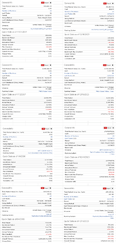
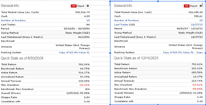
This is a follow up on view thread http://www.portfolio123.com/mvnforum/viewthread_thread,6973_offset,40 when I suggested that model designers state the number of parameters in their R2G models, but nobody supported that idea. Now we see R2G models with over 150% annualized returns and one wonders how many parameters the models have to produce such high returns.
Below is condensed from
http://gestaltu.com/2014/02/toward-a-simpler-palate.html
Performance decay occurs when the performance of a systematic trading strategy is materially worse in application than it appeared during testing.
Degrees of freedom in a system (the number of independent parameters in the system that may impact results) relates to the counterintuitive notion that the more independent variables a model has – that is, the more complicated it is in terms of the number of independent ‘moving parts’ - the less reliable a back-test generally is. This is because more independent variables create a larger number of potential model states, each of which needs to meet its own standard of statistical significance. A model that integrates a great many variables seems like it would be robust; to the contrary, it is likely to be highly fragile.
A particular model design had no less than 37 classifiers, including filters related to regressions, moving averages, raw momentum, technical indicators like RSI and stochastics, as well as fancier trend and mean reversion filters like TSI, DVI, DVO, and a host of other three and four letter acronyms. Each indicator was finely tuned to optimal values in order to maximize historical returns, and these values changed as when optimized against different securities. At one point a system to trade IWM (iShares Russell 2000 ETF) produced a historical return above 50% and a Sharpe ratio over 4.
These are the kinds of systems that perform incredibly well in hindsight and then blow up in production, and that’s exactly what happened to the IWM system to time US stocks which lost 25% in a few weeks.
The problem with complicated systems with many moving parts is that they require one to find the exact perfect point of optimization in many different dimensions – 37 for the IWM model.
It isn’t enough to simply find the local optimum for each classifier individually without considering its impact on the other ingredients. That’s because, in most cases the signal from one classifier interacts with other classifiers in non-linear ways. For example, if you operate with two filters in combination – say a moving average cross and an oscillator – you are no longer concerned about the optimal length of the moving average(s) or the lookback periods for the oscillator independently; rather, you must examine the results of the oscillator during periods where the price is above the moving average, and again when the price is below the moving average. You may find that the oscillator behaves quite differently when the moving average filter is in one state than it does in another state.
To give an idea of the scope of this challenge, consider a simplification where each classifier has just 12 possible settings, say a lookback range of 1 to 12 months. 37 classifiers with 12 possible choices per classifier represents 6.6 x 10^18 possible permutations. While a quintillion permutations may not seem like a simplification, consider that many of the classifiers in the 37 dimension IWM system had two or three parameters of their own (short lookback, long lookback, z score, p value, etc.), and each of those parameters was also optimized…
There is another problem as well: each time a system is divided into two or more states you reduce the number of observations in each state. To illustrate, imagine if each of the 37 classifiers in the IWM system had just 2 states – long or cash. Then there would be 2^37 = 137 billion possible system states. Recall that statistical significance depends on the number of observations, so reducing the number of observations per state of the system reduces the statistical significance of the observed results for each state, and also for the system in aggregate. For example, take a daily traded system with 20 years of testing history. If one divides a 20 year (~5000 day) period into 137 billion possible states, each state will have on average only 5000/137 billion=0.00000004 observations per state! Clearly 20 years of history isn’t enough to have any confidence in this system; you would need a testing period of more than 3 million years to derive statistical significance.
As a rule, the more degrees of freedom a model has, the greater the sample size that is required to prove statistical significance. The converse is also true: given the same sample size, a model with fewer degrees of freedom is likely to have higher statistical significance. In the investing world, if one is looking at back-tested results of two investment models with similar performance, one should generally have more confidence in the model with fewer degrees of freedom. At the very least, we can say that the results from that model would have greater statistical significance, and a higher likelihood of delivering results in out of sample that are consistent with what was observed in simulation.

