x Sorry was trying to put below post into here
From the paper:
Marc,
Seems like you might disagree on–at most–15% of those factors (at t ≥ 3 requirement). And even then, the authors might be the first to say that some of those 15% might not be found to be significant in another future study, for a variety of reasons. This includes the problem, as you point out, that it might not have been a rational idea (based on sound theory) to begin with. And for a number of statistical reasons including the multiple comparison problem.
-Jim
That’s pretty much why I wnt to reach out to these guys. They are spot on to be pointing out the problems with all of these factors. And I’d hypothesize that even the 15% aren’t as good as they might believe.
I’m interested in seeing research go beyond this and taking th next step . . . to understand WHY they are seein what they’re seeing. So far, nobody in the quant community seems to be understanding why. I think these professors seem to be the only ones I’ve seen in finance who might be inclined to take the next step.
Cool. For me, at my level, it is hard to look at interactions between factors without some violations of assumptions–like independence. But, I too, think this is important. Maybe you can help them with which factors might be expected to interact in a positive way and perhaps they can do a proper study of this.
Cary,
This is a great place for the post, IMHO. Thank you for broadening the topic. I am not even sure that it is really a broadening of the topic but rather it may be the exact same thing.
p-hacking in studies, alpha inflation, problems with multiple comparisons in our ports etc are all the same problem, I think. And I am pretty sure that Bayesian statistics it not going to be the only solution—if it is a solution at all.
-Jim
In the linked podcast with Wes Gray the author said they are currently trying to build a global dataset (they mentioned that building global datasets in
is notoriously hard in the academic community because the Compustat Global data is so expensive and so incomplete), to test anamolies against global markets. Once they have the ability to do that, and discount the home bias of only testing against US data they might have a better handle on the “why” questions.
It won’t get them anywhere close . . . all they’ll get is more of “what”
The why cannot be uncovered by bad sampling and going global won;the correct the problem.
Example: Some of the many factors they tested involved various measures of dividend yield. They need to know going in that they could not expect good results unless they conditioned their sample based on indications of payment risk. Similarly, value factors cannot be expected to work consistently unless they systemically condition their samples to eliminate companies whose earnings are expected to fall; companies for which low P/E etc signals bad performance. Etc. etc. etc.
Essentially, a completely different study design is needed. Maybe I’ll have to be the one to do it.
I can’t think of a single stock model I’ve built that doesn’t combine various factors in the ranking and/or the buy/sell rules. It’s almost impossible to build a port without combining at least two factors.
Unless I am missing something, I don’t see how Zhang’s research applies to the real world of building ports. Which may be what Marc is saying.
This where I agree with Marc.
When they combine variables in the literature they tend to use multivariate linear regressions.
Here is one of the assumptions (before you can do this) from SPSS: “There needs to be a linear relationship between (a) the dependent variable and each of your independent variables, and b the dependent variable and the independent variables collectively.”[/b]
(b) is an assumption that is not always listed everywhere.
Marc (for good reason) wants to put together variables that interact. I might be mistaken but my default belief is that two variables that interact will not form a line or a plane in most cases. For example, if either variable is negative there may be no interaction and no effect on the dependent variable. It is often only when both are positive that there is an interaction and an effect on the dependent variable. This shape (not a plane) clearly will not form a line with a cut (or intersection) from a plane. So not a plane and not a line.
And , I think, even the portions of the plane/line where both independent variables are positive are often more exponential than linear.
Catch 22: to meet these requirements it is usually necessary for the variables to be independent of each other—making it difficult to use this tool to look at and explore interactions of independent variables on the dependent variable. Interactions that should not exist for variables that are independent of each other.
Then there is the more often stated problems with multicollinearity. Which allows the variable to interact (a little bit) in a liner fashion: just not too much. Me I will take as much positive interaction as I can get.
As with much of this, my ability to understand my limitations is limited. But I think Marc has a point.
This much I can say for sure: like the authors I stick with the t-test (and Bayesian Equivalent).
-Jim
I have a prior that may work for 5-stock sims (and could be expanded to other sims). I simply ran a 5-stock model with random ranking and adjusted slippage so that the slippage was close to the same slippage as the sim/port I was looking at. I did this 30 times and used the mean weekly excess return for each of the 30 runs to form a prior as I did above. This is negative (compared to the benchmark) because of the slippage.
Using the above method with BEST the prior is: prior=list(muM=-0.166, muSD=0.105, nuMean=35.368) for the example sim below.
I call this the “there are few good ports prior.” And I am not sure that it is unrealistic. In fact, I think the population of all of the 5-stock ports that can be run at P123 looks almost exactly random. So, I think it may be a nearly perfect prior. But is this method useful? Is it better than a classic t-test?
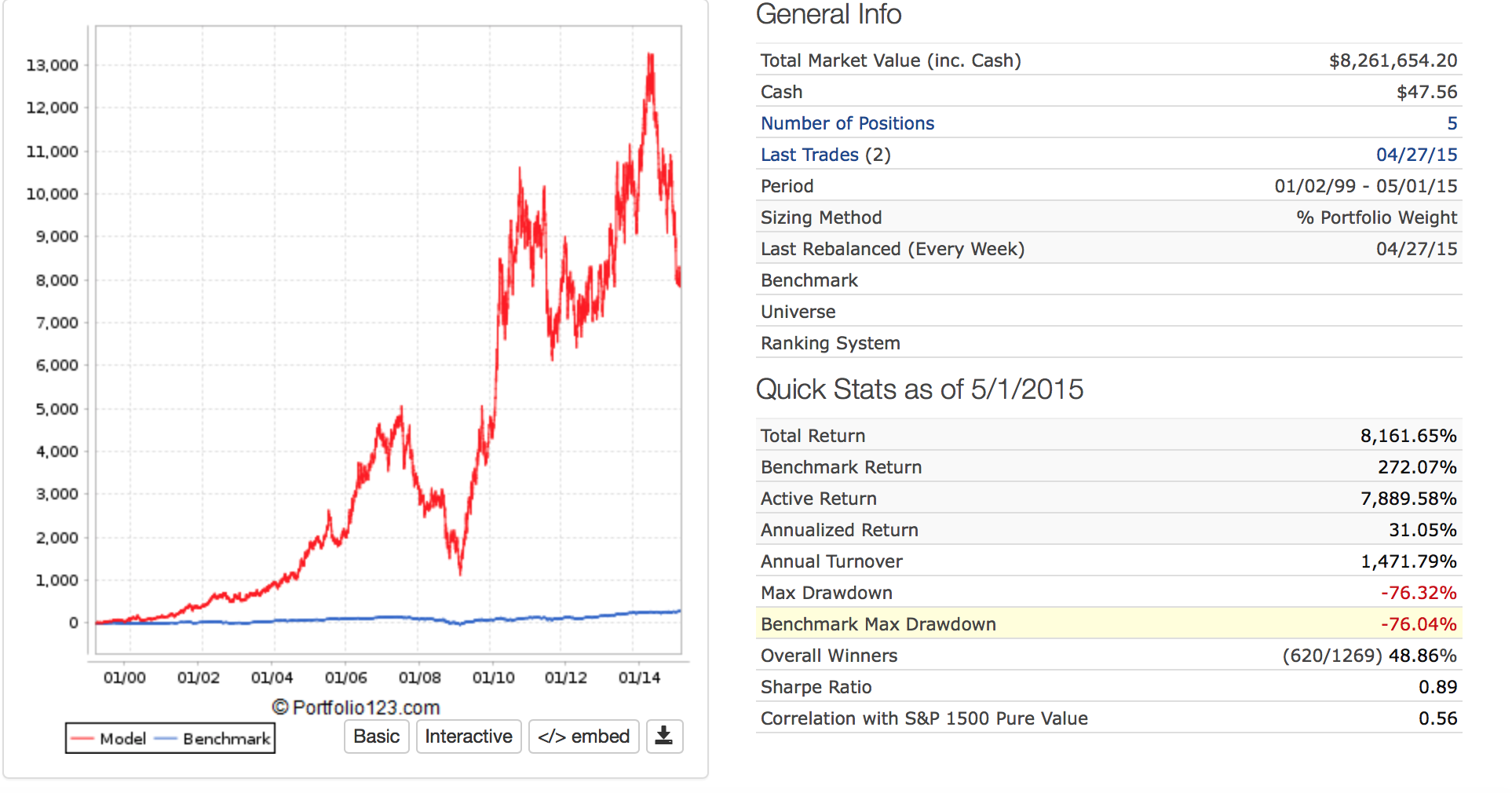
Let me show you the example of a bad sim/port and see if Bayesian Statistics raises a red flag on the sim/port. Does the classic t-test for the sim causes any concerns about the sim/port?
-
Image for in-sample sim up to 5/1/15
-
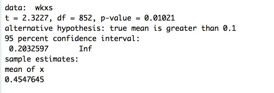
Image for classic t-test for the sim. Good right? Great p-value (p-value = 0.01021). This was done one-sided for greater than about 5% annualize excess returns per year (absolute minimum to make it worth funding a port)
-
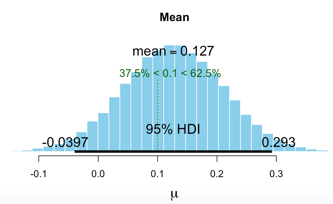
Image for Bayesian t-test (BEST in R) using above prior. Again for greater than about 5% annualized excess return. 37.5% < 0.1 <62.5%
-
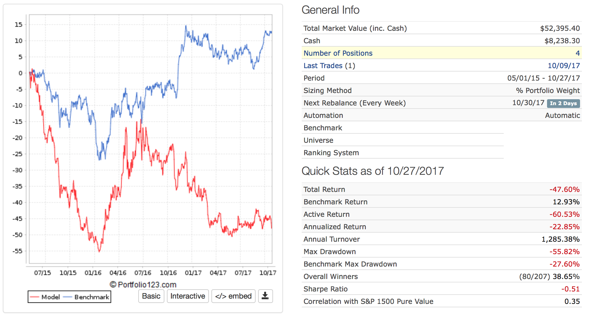
Image for out-of-sample automatic port.
The classic t-test would not have warned anyone not to fund the port. BEST (using an informed prior) would have warned you away if you had required the entire 95% credible interval to be greater than .1% (about 5% annualized). Or if you had seen that 37.5% of the credible values were below 0.1 (37.5% < 0.1 <62.5%).
I recognize there are other bad things about this port that would have raised red flags for most people at P123. I did not want to spend much time searching for other examples that did not involve my live ports. But this example–undeniably–shows the inadequacy of the classic t-test for looking at this port/sim. And there is a stark contrast between the level of significance (indicated by the p-value) and the out-of-sample results for this example.
This technique, anecdotally, tends to give a range of realistic expectations for out-of-sample results. Note that the most credible annual excess returns for this “bad port” example was about 7% with negative values being credible. This turns out being a much better estimate than either the sim or the 95% confidence interval for the t-test. 7% annualized excess returns was not even in the 95% confidence interval of the t-test (0.203 to Inf).
This is looking like it might be a useful technique. It may begin to address problems with alpha inflation, p-hacking, and with multiple comparisons. It may give more realistic exceptions for out-of-sample result. Potentially, this technique—along with other established techniques—could help avoid funding of ports that dramatically underperform out-of-sample. Nothing can completely remove this problem.
When it comes to investing, I will use anything that improves my “batting average.”
-Jim
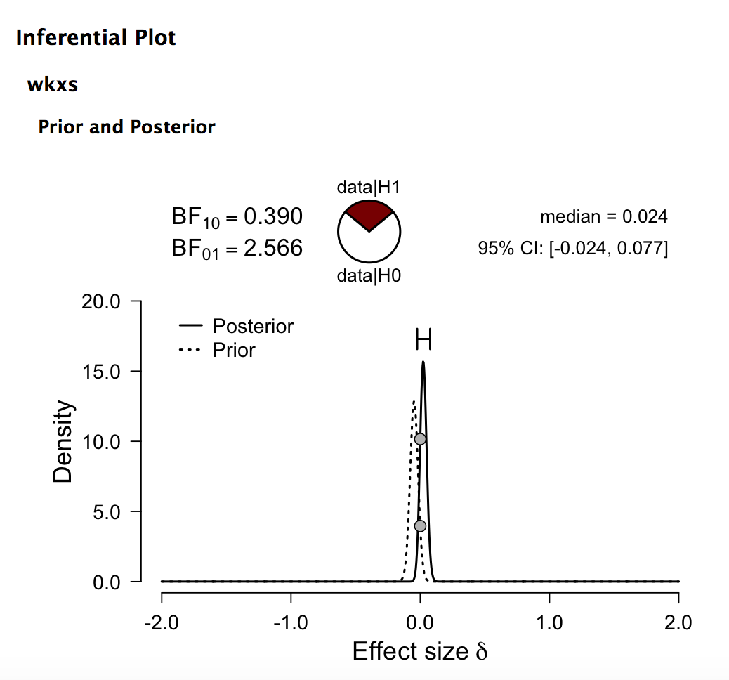
To be complete I should probably give the results of a Bayesian t-test.
The above is called Bayesian Parameter Estimation: using an informed prior in this case.
The reason this is worth posting is this: Bayesian Parameter Estimation raises a red flag and would make one take pause before funding the port.
The Bayesian t-test strongly argues agains funding the port! The Bayesian t-test says the odds of the port being a good port are less than 1 (0.390). JASP gives a Bayes Factor of 0.390 in favor of alternative hypothesis (that the true parameter is not 0). Or the odds of the null hypothesis being correct (parameter = 0) of 2.566.
Using a Bayesian t-test if often called “model selection” which, I guess, is what we are trying to do. “Model” here means best “model” for stock/port behavior which, again, is probably what we are trying to do.
Despite the apparent advantage of the Bayesian t-test in this example, I am not sure that I do not prefer the Bayesian Parameter Estimation with the requirement that the 95% credible interval not include a specified parameter (5% annualized in this example). However, setting the parameter to 0 for this or a classic t-test is problematic as you are likely to find significance for very small effects with large data sets. In this example, anything less than 5% annualized is considered a small effect and is “practically equivalent” to zero in Bayesian parlance.
The Bayesian t-test gives you very conservative results and is likely to keep you away from bad ports with a strong likelihood that any ports you do invest in will work.
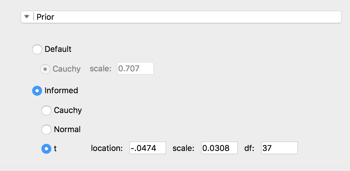
For those with an interest: the ratio of the prior density and the posterior density at 0 is called the Savage-Dickey density ratio and it has been an integral part of all of the Bayesian t-tests beginning with Harold Jeffreys who developed the Bayesian t-test in 1935. JASP is one of the few programs that allows the use of a t-distribution for the prior. I am not aware of an R program for a Bayesian t-test that does allow for the use of a t-distribution prior. BayesFactor for R uses a Cauchy distribution: which turns out to be a t-distribution with nu, or the degrees of freedom, set to 1.
JASP uses the effect size so I have adjusted the t-distribution for this (obtained using BEST). See the images.
The only thing better would be a time machine!
BTW, thank you community for tolerating this large post!!! I would not have thought of the idea of using a random prior with slippage for sim priors if I had not been putting my ideas into writing. I hope this may be of some use to some in the community. Personally, I think some method of dealing with the fact that we are running a lot of sims–until we get what we want–is a must. That method does not have to be Bayesian Statistics but it might be one method that works and there is a theoretical basis for thinking that it should.
-Jim