Moneyball, Batting Averages and Stock Returns

I find myself asking what Billy Beane would do. As you know Billy Beane—as played by Brad Pitt in the movie Moneyball—produce a winning baseball team by using statistics to help with decisions about player recruitment. This is based on the real-life Billy Beane. If I could be as successful as Billy Beane and as cool as Brad Pitt…….

Note: Marc was the first person to make the analogy of what we do to Moneyball. I am hoping he will not mind me borrowing this analogy if I give him the credit he deserves.

I came across this free PDF about predicting future batting averages for a player (or the ‘True batting average’). Link here:[url=https://gumroad.com/l/empirical-bayes]https://gumroad.com/l/empirical-bayes[/url]

The author of this PDF asks the question: who is the best batter? All of you who follow baseball know that the best batters are: Jeff Banister, Doc Bass, Steve Biras, C.B. Burns, and Jackie Gallagher.

These are the players with perfect batting averages and therefore must be the best players, right?. And they must be in the hall of fame, right? Never mind that these players all had only one or two at bats.

Hmmm. Best batting average but not necessarily the best batters—and no they are not in the Baseball Hall of Fame for hitting. We all make an adjustment with small samples naturally. Is there a quantitative way to make such an adjustment?

The PDF uses Empirical Bayesian Statistics to determine what the true abilities of the players in the major league are. And he answers the burning question: does Hank Aaron belong in the Hall of fame? I think it is worth a read to give a better gut-feel on how to make adjustments for outliers, small samples, cherry-picked data and the multiple comparison problems. This PDF is readable. Just ignore and details about the beta function. I refer you to “Doing Bayesian Data Analysis” by Krutschke for a more detail example of batting averages and Hierarchical Bayesian Analysis wth multiplies levels. Multiple levels are good for questions like: what if the player is a pitcher?

This can be done with stock returns too. I will go through the rest quickly.

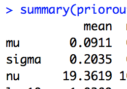
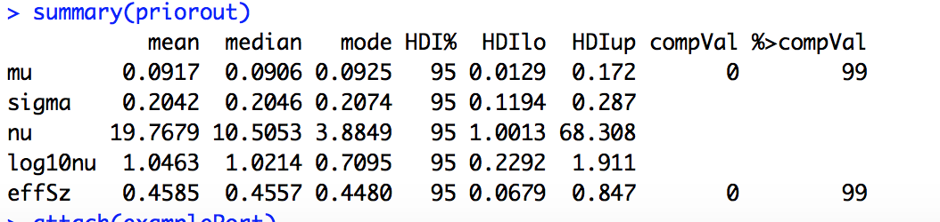
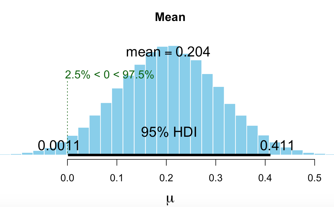
The PDF develops a prior for batting averages. I develop a prior by finding the weekly averages for all of my ports including a number of unfunded auto ports. See first image for the t-distribution for the prior generated by BEST in R.

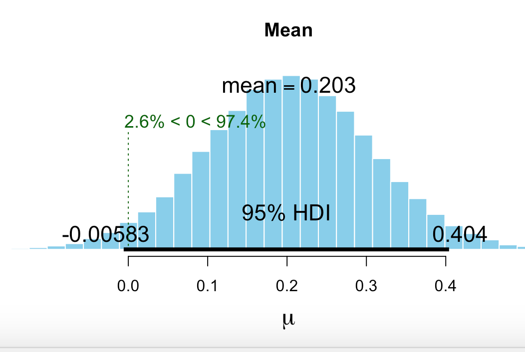
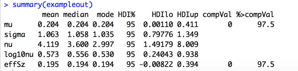
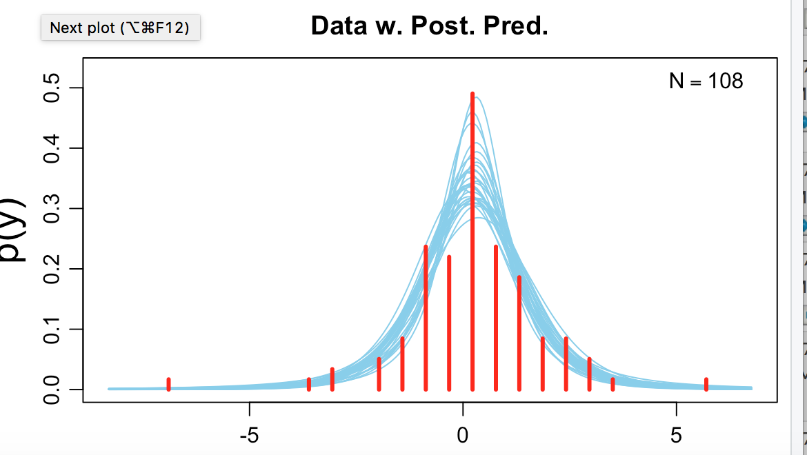
The PDF then generates the posteriors for the players including Hank Aaron. Billy Beane could have had to decide whether to add Hank Aaron to the team (or how much to offer him). I have to decide whether one of my auto ports should be funded. See the posterior probabilities for excess returns for one of my auto ports.

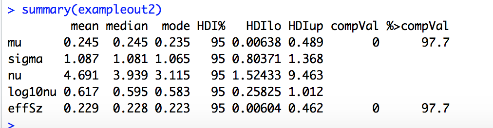
The most credible value for excess returns is 11% for the port (annualized). The 95% credible interval just barely includes zero.

You can make your own judgement but only 11% better than the benchmark and not quite significant based on the 95% credible interval? Hmmm… Using the prior for this port did not cause a huge correction (shrinkage in the Bayesian parlance) for this port but it did for the ones with more extreme excess returns.

What would Billy Beane do? Maybe not this exactly. But he would not pay a lot for Doc Bass’ batting skills. And he would use something like this: he wouldn’t just relying on his gut, I think.

This could be adapted to selecting Designer Models with objective criteria for selection.

-Jim


Prior.png


This is very interesting. If you are doing this in R would you mind posting the code as I would like to learn how to do this?

I bought the book.

In building a portfolio, you have to consider how the models correlate with one another. To use the baseball example, you want hitters who get on base batting before your power hitters so the power hitters have more RBI opportunities.

Correlations and volatilty are easier to predict than returns. Multiplying monthly SD by the square root of 12 vastly understates actual annual volatility by the way. Run monthly rolling annual returns of your ports and see for yourself.

We’ve gone to selecing ports with a minimum excess return profile that are not overly correlated, and weighting those ports by the amount of risk they pose. Risk parity so to speak. In this way, we are agnostic as to predicting which port will outperform. We monitor the ports to make sure they are operating within expected bands. We have noticed a genereal mean reversion pattern in the ports, so from time to time, we trim outperforming ports and add to underperforming ports.

It’s the KISS method.

Fascinating topic . . . yes I did make the moneyball analogy.

Billy Beane is well known, but particularly interesting are what we learn in the years since he broke onto the scene. Paul DePodesta, Beane’s right-hand man at Oakland, went, as many know, to the Cleveland Browns to bring serious analytics to that woebegone franchise. His job was easier. The NFL has long been into serious analytics for game strategy - it was just a matter of applying it to roster building. And, the NFL has a salary cap so the Browns are just as financially able as any other team, unlike the Oakland A’s. also, the Browns were loaded with top draft picks and knew they could pretty much get any player they decided they wanted. As an analytics fan in general, I decided to start following the Browns and set them as one of my favorite teams in my ESPN.com settings.

So far, though, it’s been a disaster, worse than even the most pessimistic person could have imagined. They had QB Carson Wentz right in their hands. They traded the pick away becaase the analytics team decided Wentz would not succeed in the NFL. This past draft, DeShaun Watson was available to them, head coach and QB guru Hubie Brown wanted him and even texted him before the draft to “be ready.” The analytics team rejected Watson and went of Deshaun Kizer instead.

As it’s been turning out, Wentz and Watson are looking like franchise altering star QBs and it looks as if, despite the Browns; owner’s stated desire for patience and stability, like there is housecleaning on the horizon and the general though is that the analytics experts will be fired.

Not sure if all the current Browns rumors are true. Their defense is terrific, though a lot of that may have something to do with the hiring of fire-and-brimstone Greg Williams as the new defensive coordinator. But one thing is very clear. Analytics, divorced from “domain knowledge” doesn’t the work. Billy Beane did well because he had plenty of domain knowledge. He was a highly touted major league prospect who failed horribly when he got to the majors and he studied specifically where the scouts went wrong in evaluating him, and developed his ideas around how his own lack of major league talent should have translated into measurables. Not sure DePodesta could have accomplished anything without the ex ballplayer in his ear and over his head. Clearly, in Cleveland, DePodesta needed to be talking to and leaning from his QB guru coach rather than dictating to him from on high.

There are also other un-studied issues in baseball analytics. The main one emerging now is whether the models that hel build a winning team can get a team that can survive post season, where the parameters are very different. The weather is colder. And the compressed critical nature of each series means players, especially pitchers, have to change roles; closers may need to go more than an inning. Starters often need to come out of the bullpen, etc. In the regular season, wins and losses is a probability game and a team can take many losses in the name of long-term benefit. In post season, each loss is a crisis and possibly an elimination.

These same principals apply to our analytics. They can and do work. They helps us see things not otherwise visible and give us fortitude to know when seemingly important things can be dismissed as trivial. But analytics in isolation can’t work. In Cleveland, they call it an epoch embarrassing QB misses. The Washington Nationals are calliing it pitching mismanagement, although so far, the are still getting away with blaming the manager. Here, we call it data mining.

No matter how statistically sound your p123 statistical work, just make darn sure that you don’t pass on Carson Wentz or DeSuan Watson.

Miro, thanks for the great points. This really is equivalent to predicting mean reversion. It requires less data than than would be required do it using formal mean-reversion techniques. Of course, just because you have a prediction of mean-reversion it does not mean the prediction will be right.

To predict the returns–using mean-reversion–in 2 years would require 4 years of data. First 2 years (out of the 4) on the x-axis and last 2 years on the y-axis. Then you could predict the reversion of the next 2 years using this data. This Bayesian method requires only 2 years of out of sample data.

Great points and I appreciate your comments. I will spend some time thinking of each of your comments in depth.

@Shaun: I will send the code and screen-shots. Very, very easy if you have used R before: coming.

-Jim

Jim,

The pattern I’ve noticed is that when a port is suffering a drawdown faster than SPY, and then starts to recover such that the drawdown becomes smaller than SPY (the port drawdown line crosses above the SPY drawdown line), that’s a great time to reallocate to (or reactivate) that port.

As an illustration:

Parker,

Ah yes, I figured that was what you meant on the second read through of your post (but did not edit my comments). And of course, I do not see how my post could help with this.

Depends, however, on whether you are using a time-series or stationary data. It would not be reversion-to-the-mean for stationary data. It would, I think, be an actual reversal which is different. For stationary data and regression-to-the-mean, negative returns would still be negative: just not as negative. That is what I was thinking about when I responded to your excellent post.

Time-series are not in my skill set at this time. But I think you are right about the reversal (whatever one calls it) working.

@ Marc: that was so cool!!! Remind me not to take the spread on any of your sporting bets.

-Jim

Shaun,

Your R skills have to be better than mine (how could they be worse). I could not compile this into a single source code but had to break it up. Using the output from one run to enter the priors in the next. But here it is:

For each port I went to Statistics>Performance. I clicked radio button “Chart Data Weekly” and downloaded “Weekly Returns Since…” into Excel. I did this for all of my ports and entered the mean for each port into a column. I saved the data in spreadsheet priorExample with column heading priorMeans. This is the prior data. I did the same for the port of interest for posterior data. Excel spreadsheet examplePort with “example” column heading.

Download BEST package into R. There are dependencies for this. Seemed like a headache but executed the first time following the PDF directions for ??BEST in R.

I then downloaded examplePort and priorExample (CSV format).

attach(priorExample)
priorout=BESTmcmc(priorMeans)
summary(priorout)
attach(examplePort)

BREAK here to enter summary output into priors You will use your own prior data

priors=list(muM=.0912, muSD=.2034,nuMean=19.7)
exampleout=BESTmcmc(example, priors=priors)
plot(exampleout)
summary(exampleout)

Also of interest:

plotPostPred(exampleout)
plotAll(exampleout)

Note the posterior plot is slightly different. This is a property of the Markov Chain Monte Carlo giving a slightly different answer on this run.

Hope this helps and happy to clarify.

-Jim


So far this season, I’ve been a disaster on draft kings, but I’ve got strong exposure to the Eagles tonight, so this may turn into a good week, which is looking decent thus far.

The BEST package loaded fine. So you downloaded weekly returns for many portfolios and calculated the mean and sd of each and then did same for a single portfolio? I may have to read the reference before diving into this. My hope is that it will help me to do a rolling test of whether conditions have changed and the returns being generated now are sufficiently different than the priors that I should reduce capital to that strategy.

Shaun,
Way easier and way cooler than that with this amazing program. The reference is very good and should fill in where my explanations fall short. Some of the non-informative prior stuff is a little dense, however. You are not interested in the uninformative prior so skip that.

You literally just download the means of your weekly returns (for multiple ports) into one column for your prior. These means are then fit into a t-distriubtion and gives you the parameters for the t-distribution (mean, sigma and degrees of freedom or nu) in the summary. This is done by the program and you do not need to calculate the standard deviation yourself.

The image of the graph is the histogram for all of the weekly mean returns (red). The blue curves are curves fit by Markov Chain Monte Carlo. The summary has the mean, standard deviation and nu (degrees of freedom) for the fitted curve. The plot is the graph of curve (with parameters in the summary) with the histogram of your data.

So the summary for the prior (from the single column of all of the means for multiple ports) gives the the parameters for the prior.

Entered into priors=List(muM=.245, muSD=1.087, nuMean=4.691)
Then run posterior=BESTmcmc(data, priors=priors)

These are from the left column of summary under mean (image 1). muM=mu, muSD=sigma and nuMean=nu.

Actually this is other data but the histogram and the fitting of the curve to the histogram is the point.

Not easy and I read all of Kruschke’s text but worth sticking with, I think. The program is amazing and using priors is where Bayesian statistics really becomes useful.

-Jim


It’s sinking into my pumpkin. Thanks.

Hey, I am not the only one autistic enough to try this. I was Googling ideas in the attempt to define a suitable prior for sims (not just my ports). I already have some ideas but they are not ready from real money (for sure).

There is a post on Quantopian that does some of the same things I did in my post. Note she uses the t-distribution with mu, sigma and nu as defined by the R program (BEST).

Reading this post, I feel like she is making this inaccessible on purpose, however. This is in contrast to the batting average PDF I linked to. I will give her the benefit of the doubt: maybe it is just shorter because it is a post and just compressed.

But the points from accessible portions of the post are: if you can define (what you think is) a good prior then the use of a t-distribution with mu, sigma and nu (as done by Best in R) for the prior is valid. And other people are using Bayesian Statistics to analyze stock models.

The devil is in the details: what is a good prior? There can be honest disagreement on this when forming a prior. Even with Designer Ports for example, there is the survivorship bias to worry about.

Link: [url=https://blog.quantopian.com/bayesian-cone/]https://blog.quantopian.com/bayesian-cone/[/url]

-Jim

Jim

Forgive me if you have addressed this. But because of the market problem (see below), wouldn’t it be helpful to build Bayesian cones on excess returns compared to the benchmark in addition to (or instead of) cones based on nominal returns?

PS There was another Quantopian study by Thomas Wiecki (All the Glitters is Not Gold) which looked at all sorts of in-sample statistics to sort which were most predictive out-of-sample. 95/5 tail risk ratio was the most predictive of out-of-sample Sharpe ratios. Kurtosis was predictive well. In addition, volatility based metrics such as standard deviation and max drawdown were stable across in-sample and out-of-sample periods.

Jim, does your Bayesian analysis take any of these factors into account?

Parker,
I agree 100%. Honestly, I cannot follow her post very well at this point. I will read it until I understand it better. I’m thinking her “cone” corresponds (somewhat) to the 95% credible interval in my post but I am still studying it. I am only endorsing the use of Bayesian statistics (if you have a good prior) and the t-distribution from her post at this time.

But everything I did with my ports is 100% excess returns.

You are absolutely correct in my opinion–one reason I voted for the information ratio feature request :wink:

-Jim

Parker,
Short answer: no. The returns for my ports including the ones on auto is the first thing I tried. Partly, because it is the only complete, not cherry-picked with no survivorship-bias sample I could think of at the time.

I think Designer Models is probably a good enough sample and I was going to post something on that but I did not want to endorse/embarrass anyone.

Priors for sims to address the multiple comparison problem is what I would like to be able to do in the future.

-Jim

This is a good a place to drop this as any, I would be interested in hearing people’s thoughts on this.

Wes Gray at Alpha Architect on Kewei Hou, Chen Xue, and Lu Zhang recent academic paper on Replicating Anamolies.

https://alphaarchitect.com/2017/10/26/want-to-learn-more-about-factor-investing-read-this/

Wes Gray interviews Lu Zhang on his research on the Behind the Markets Podcast on Factor Repliction.

https://alphaarchitect.com/2017/10/16/32859/

They are correct in that returns from anomalies are concentrated in small cap stocks.

Academic studies often do not consider transaction costs, market impact of trading, short borrow availability nor cost. The time scale can be deceptive especially when the alpha decay is material an many such studies use annual rebalancing, though the better ones do monthly.

His preferred set of factors can be turned into a reasonable screen and there are 50 ways to skin that cat.

x

I looked at the factors they studied. Microcap issues aside (and I say “aside” loosely because microcaps exist and play an important role in the market, I didn’t see any factors that could logically be expected to be predictive of future returns, and some (a series of dividend yield factors) that should be predictive of poor returns.

It’s the standard study-design problem about which I’ve often written. No factor has any meaning in isolation. A factor can only be useful when appropriately conditioned. Essentially, these studies are sampling incorrectly. Qunats have consistently been suffering from inadequate domain knowledge which is preventing them from realizing that they should be working with “purposive sampling.”

I’m going to reach out to the authors and try to engage them on this issue. They seem to have a deep interest in it, and less emotional commitment to the standard fama french doctrines, so maybe they might be open to trying to take research into a different direction. Maybe it will help that two out of the three authors are at Ohio State, my alma mater. Go Buckeyes!!!