Regression functions and smoothed factors now available

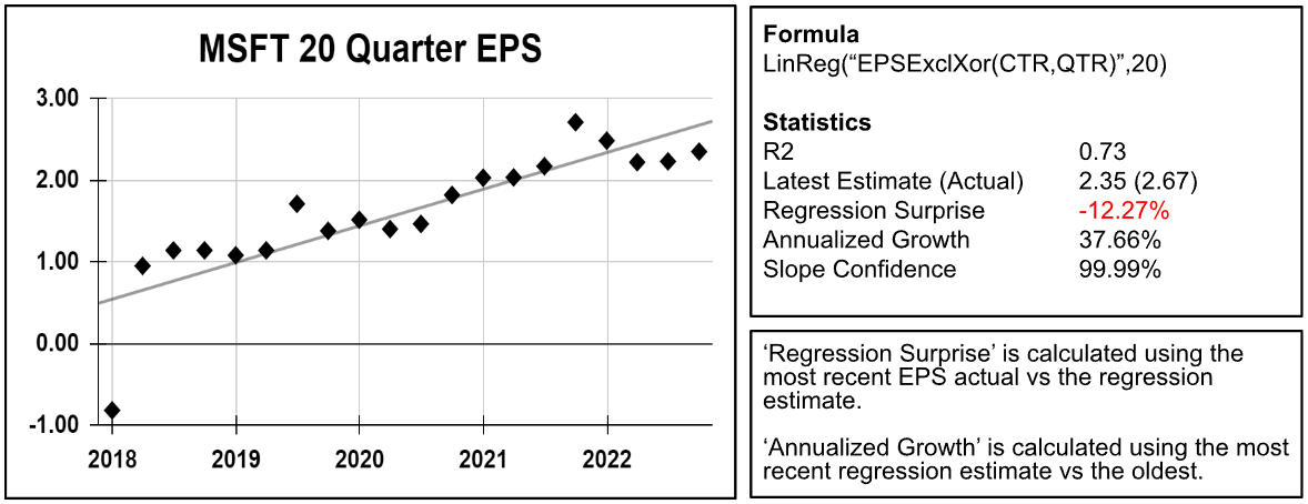
A complete set of regression functions and factors are now available for screening and ranking. These are a great way to deal with outliers. Below is an example with Microsoft’s 20-quarter EPS regression. As you can see the growth rate of 37.66%, calculated using the regression, is not affected by the 2018 outlier.

Some of the things you can do with regressions include:

  • Find stocks that have a positive EPS slope (growth) with a good fit (low volatility).
  • Rank stocks based on their combined regression statistics: slope, R², and growth.
  • Find stocks where the latest EPS is above or below the regression estimate.

To use regression functions, you will need an active Ultimate or higher membership (or equivalent). You can also use regressions during a 21-day trial.

You can find all relevant documentation and examples in the factor reference.

Below are some examples and excerpts from the documentation. We hope you find these new features useful. Please let us know if you have any questions!

Cheers,
The Portfolio123 Team

Examples

To use regression, you need to use a LinReg function, then you can use factors to access the statistics. Multiple regression in your formulas are allowed using precise placement: regression factors access the most recent regression formula preceding the factor.

Time Series Regression

To find stocks where the 10Y sales regression has: 1) a positive slope 2) a good R2 of at least 0.8 and 3) latest sales above the trend, you could type the following

LinReg("Sales(CTR,ANN)",10)
R2 > 0.8 and Slope > 0 and SurpriseY(0) > 0

XY Regression

To find company where the latest EPS is above the expected EPS for a given revenue you could do the following:

LinRegXY("Sales(CTR,ANN)","EPSExclXor(CTR,ANN)",10)
SurpriseY(0) > 0 

Spreadsheet calculation

Click here to open a spreadsheet example of all formulas

FORMULA FUNCTIONS ➞ REGRESSION FUNCTIONS

The following functions evaluate a regression:

LinReg(“Formula(CTR)”, iterations )
LinRegVals(y0,y1, …. y50)
LinRegXY(“X-Formula(CTR)”, “Y-Formula(CTR)”, iterations)
LinRegXYVals(x0, y0, …, x50, y50)

The first two are time-series regressions where the X is not supplied and represents a period of time. The “XY” regressions are general regressions where the X is explicitly supplied.

FORMULA FUNCTIONS ➞ REGRESSION STATS

The following statistics are available after you calculate a regression:

R2, SE, Slope, SlopeSE, SlopeTStat, SlopePVal, SlopeConf%, Samples, Intercept, InterceptSE

These statistics have a parameter

SurpriseY( offset ), EstimateY( offset ), EstimateXY( X ), RegGr% ( period = 1 )

PREBUILT SMOOTH FACTORS

For every fundamental line item you can find predefined regression factors for the most recent estimate and for the annualized regression growth. We predefine them for two periods: 5Y of TTM values sampled every 6 months and 10Y of Annual values. You will find these Smooth factors in the reference of each line time. For Example these are the Smooth factors for “Sales”

Prebuilt regression factors are available for any membership.

Factor Equivalent to
SalesRegEstTTM Eval(LinReg(“Sales(CTR * 2, TTM)”, 10), EstimateY(0), NA)
SalesRegGr%TTM Eval(LinReg(“Sales(CTR * 2, TTM)”, 10), RegGr%(2), NA)
SalesRegEstANN Eval(LinReg(“Sales(CTR, ANN)”, 10), EstimateY(0), NA)
SalesRegGr%ANN Eval(LinReg(“Sales(CTR, ANN)”, 10), RegGr%(1), NA)
3 Likes

Oh, this is very nice. Thanks!

1 Like

Just a few explanations in case anyone’s confused.

Here’s how to use these. In a screen or simulation or aggregate series, you’ll need to use the LinReg function on one line and then call up the stat (or stats) on any line below it. Or you can use an Eval statement as follows: Eval (LinReg (“formula(CTR)”,iterations), stat, NA). You can also use that Eval statement in a ranking system; alternatively, you can add a node with the LinReg function with 0% weight and then follow it with a node with the stat you want.

A few words about the stats:

R2 measures the goodness of fit and ranges from 0 to 1. It does not tell you whether the line slopes up or down.

Slope is measured per period. So if you’re measuring the slope of quarterly EPS and you get 0.05, that means that the company’s EPS is going up five cents per quarter. If you’re measuring annual sales and you get -150, that means that the company’s sales are going down $150 million per year. You therefore might want to use the RegGr% function or scale the slope by the average if you’re comparing things like EPS or sales. You don’t have to do that if you’re measuring changes in ratios like ROA or profit margin.

RegGr% takes the difference between the first and last estimates and divides that by the absolute value of the first estimate, then compounds that value per the period specified.

EstimateY will tell you what the regression line estimates for a specific period. You can also use EstimateY to tell you what the regression line estimates for periods outside your sample (in the future, for instance). SurpriseY will tell you how the actual value compares to the estimated value.

More advanced stats are also available. If you’re familiar with regression stats, you’ll be able to use standard error (SE), T-stat, P-values, and more.

Linear regression fails if there are any NAs in the series.

Have fun!

2 Likes

OK, now I’m sad.

“To use regression functions, you will need an active Ultimate or higher membership (or equivalent). You can also use regressions during a 21-day trial.”

So Legacy subscribers are cut out?

Legacy memberships that cost around the same or more than Ultimate can also use regression functions. Keep in mind that switching to Ultimate will not reset your start date, so you will likely not lose any history. For example if you have had a continuous membership since 2017 , moving to Ultimate would give you 20Y since 2017. In other words the entire history.

And “smoothed” factors are available for any membership.

1 Like

Well, I’m in the “Designer (Legacy)” group and that doesn’t appear to close enough. Oh, well. I’ll consider an upgrade.

Thank you Marco. It looks powerful with a lot of potential uses.

So many new possibilities, I don’t know where to start!

1 Like

This is absolutely fantastic… I have a lot of work to do. Cheers!

R2 measures the goodness of fit and ranges from 0 to 1. It does not tell you whether the line slopes up or down.

This is, sadly, not true. A while back I wrote a short article with examples illustrating why R2 is both not a predictor of the expected performance / accuracy of a model: R squared Does Not Measure Predictive Capacity or Statistical Adequacy - KDnuggets

Though observational studies are only a side interest for me so far, I think it is best interpreted as an estimate of the percentage of the variance explained by the regression variables, assuming the model fits.

Regardless, these are very welcome additions! I’ve wanted something like this and so I’ll be playing a lot with these new functions in the following days.

EDIT: Removed an incorrect statement: “nor is it a measure of goodness of fit” above. I think I’ve confused the intended application of R^2 due to my background in which goodness-of-fit tests are typically used for checking model assumptions, whereas in regressions R^2 is typically used as a measure of goodness-of-fit after establishing model assumptions hold. I apologize for putting words in Juval’s mouth.

From your article

The standard error would have been a much better guide being roughly seven times smaller in the first case

But standard error is in the Y units so not good for ranking in most cases (Sales, EPS, etc). Anything else we can add that is unitless (therefore rankable) that measures fit?

Thanks

There are a lot of ideas in article below but a lot of the formulas seem wrong https://www.analyticsvidhya.com/blog/2021/10/evaluation-metric-for-regression-models/

Geoprofi,

I have recently (before your post) reviewed this. This is an interesting topic.

As I am sure you know Python has a completely different way of calculating the R^2 with some theoretical advantages.

In words, it compares how well taking the predicted value of the regression did compared to how you would have done just taking the mean as your predicted value.

Link here: Sklearn R^2

As you know R^2 can be a negative number over at Sklearn meaning you can have an infinitely bad model and Sklearn will let you know it. This goes beyond considerations regarding the slope of the line and includes non-linear considerations.

Ultimately, Isn’t that what you really want to know: Is going through all of this math and coding better than just taking the mean? And honest feed back can be good, especially if your model is infinitely bad.

That having been said, I have found the R^2 as calculated in Excel useful and not totally without merit.

I look forward to the time when geoprofi and others can have a conversation with the person developing AI at P123 and maybe after some discussion at least consider tweaking —or adding to–some of the metrics (when warranted).

Edit: Here is the code if anyone wants to play with this R^2. From the Excel spreadsheet form a column of the real values and the predicted values (‘Observation’ and ‘Predicted’ respectively in the code) and save as a new spreadsheet, RSquared.csv and upload this spreadsheet in Python using this code (for a Mac):

import pandas as pd
df = pd.read_csv(‘~/Desktop/RSquared.csv’)
from sklearn.metrics import r2_score
Observation =df[‘Observation’]
Predictedr =df[‘Predictedr’]
R_square = r2_score(Predictedr, Observation)
print(‘Coefficient of Determination’, R_square)

Jim

Hi Marco,

As mentioned, observational statistics like regressions and ARIMA are but a side interest of mine at the time of writing. I’m used to working with data obtained from randomized controlled trials and for these goodness-of-fit measures and tests of various assumptions regarding the data-generating mechanism work reasonably well (though they lack in statistical power with low sample sizes such as the ones one can often encounter in econometric data).

With that disclaimer out of the way, my understanding is that an examination of the plot of residuals is the preferred way to check for the statistical adequacy of a model. Since residuals represent the error term they should exhibit characteristics related to the chosen model, e.g. in a simple Normal IID model:

  • normally distributed
  • constant mean (mean-homogeneity)
  • constant variance (homoscedastic)
  • independent observations

The moments of the residual distribution by themselves would not do, one needs to examine the various assumptions with relevant tests, e.g. a battery of tests of normality for the N assumption, tests of independence for the independence assumption, and so on via auxiliary regressions where necessary. With significantly flawed model fits, a simple look at the residuals would immediately make any patterns visible (such as the illustrative models in my article).

Hope this is helpful and correct.

Jrinne,

I’ve practically zero experience with Python so I’m not aware of any of its peculiarities. The mentioned R^2 method from the SKlearn library seems rather different than both the standard definition of Pearson’s R^2 and methods implemented in other Python libraries such as scipy.stats.linregress where it is computed in the classical way.

I’m certainly not saying R^2 is without merit - it does what its description says and can even be used as a goodness-of-fit measure assuming the model is well-specified. It should simply not be used as a measure for the statistical validity of the model. Revisiting both Yuval’s statement and Marco’s question in this sense I might have read too much into what they mean by goodness-of-fit (confusion of application) as I’ve typically seen it as part of ensuring the statistical validity of a test, whereas in certain applications of regression “goodness-of-fit” takes a meaning on its own and statistical validity is assumed to have been established before reporting and interpreting an R^2.

geoprofi,

I think your comments/observations are spot-on and 100% accurate. I am learning about this and Python’s method is just something I have looked at recently: Precisely because you are right about what you have said.

I appreciate your comments and hope they will lead to discussions and continuous improvement in P123’s AI.

Best,

Jim

Have any of you improved a ranking system by using these new regression functions?

1 Like

I’m confused; perhaps I’m just missing it.

I only see one variable in these functions. Can someone tell me what these independent and dependent variables are in these regression functions?

Hi, Might be easier to clarify if you can describe what you are trying to do? Thx

For starters, I’m trying to see / test these new functions. I need to understand what’s being regressed with the regression function (i.e. what we are trying to explain using ordinary least squares methodology). Like, all these outputs are measuring what exactly?

For me, I thought users select the one (more) independent variables that will explain one variable in the database. The dependent can be anything - the stock price, the stock return over x days, the volatility over X days, sales growth over X days, etc. The factors that “explain” any one of those things. Maybe it could be a ranking system, as an example.

The independent variable is the period. For example, LinReg(“Sales(CTR,ANN)”,10) regresses the last ten annual sales figures against the numbers 0 through 9, with 9 being the most recent period. See the examples here: Regression Example - Google Sheets

You can also choose your own independent variable using LinRegXY.