It tried but...
Trending versus Mean Reversion in Factor Returns: A Technical Analysis
I analyzed the weekly returns of the top bucket for 31 different stock market factors to investigate their predictive properties. The key finding: weak predictive relationships (three statistically significant) with mean reversion dominating. NOTE: you would expect a few statistically positive tests of 31 factors, with multiple window sizes tested, by chance alone.
Methodology:
- Tested if the SMA over a period predicts average returns over the next 4 weeks
- Grid search for optimal SMA window sizes: [4, 8, 12, 16, 20, 24, 28, 32 weeks]
- Used linear regression to test predictive power
- Analyzed correlations, p-values, and statistical significance
Key Findings:
-
Evidence of weak predictive relationships:
- Correlations range from -0.0880 to +0.0339
- Three factors show statistical significance (p < 0.05)
- 21 of 31 factors show negative correlations (mean-reverting tendency)
- All best performing windows were 4 weeks
-
Window Size Analysis:
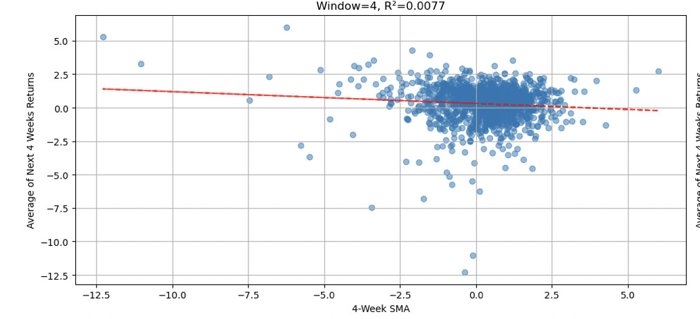
- 4-week window emerged as optimal for all factors
- R-squared values all below 1%
- Predominantly negative correlations suggesting mean reversion
Results table (name of factors removed):
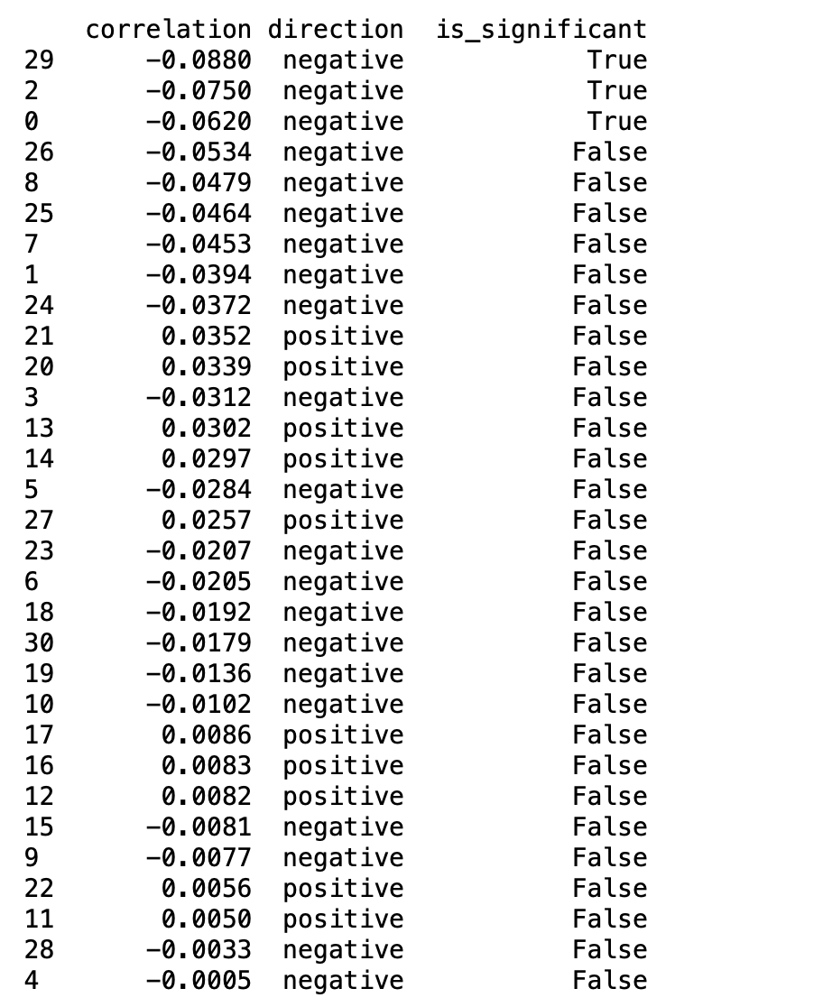
Most significant regression results:
Code included for transparency and replication.
import pandas as pd
import numpy as np
from scipy import stats
import statsmodels.api as sm
import matplotlib.pyplot as plt
import seaborn as sns

def analyze_predictive_power(data_series, window):
    """
    Analyze predictive power of SMA for average of next 4 weeks' returns
    """
    # Calculate SMA
    sma = data_series.rolling(window=window).mean()

    # Calculate average return over next 4 weeks
    forward_returns = pd.concat([data_series.shift(-i) for i in range(1, 5)], axis=1).mean(axis=1)

    # Remove NAs from both series
    sma = sma[window:-4]  # Remove first window periods and last 4 periods
    forward_returns = forward_returns[window:-4]  # Align with SMA

    # Run regression of forward returns on SMA
    slope, intercept, r_value, p_value, std_err = stats.linregress(sma, forward_returns)

    # Calculate correlation
    correlation = sma.corr(forward_returns)

    return {
        'window': window,
        'slope': slope,
        'p_value': p_value,
        'r_squared': r_value**2,
        'correlation': correlation,
        'std_err': std_err,
        'direction': 'positive' if slope > 0 else 'negative',
        'is_significant': p_value < 0.05
    }

def analyze_all_metrics(data, windows=[4, 8, 12, 16, 20, 24, 28, 32]):
    """
    Analyze predictive power for all metrics
    """
    all_results = {}
    significant_predictions = []

    # Analyze each column
    for column in data.columns:
        if column != 'date':
            print(f"\nAnalyzing {column}...")

            # Test each window size
            window_results = []
            for window in windows:
                result = analyze_predictive_power(data[column], window)
                window_results.append(result)

            # Convert results to DataFrame
            results_df = pd.DataFrame(window_results)
            all_results[column] = results_df

            # Track significant predictions
            best_window = results_df.loc[results_df['r_squared'].idxmax()]
            if best_window['is_significant']:
                significant_predictions.append({
                    'metric': column,
                    'window': int(best_window['window']),
                    'r_squared': best_window['r_squared'],
                    'direction': best_window['direction'],
                    'p_value': best_window['p_value'],
                    'correlation': best_window['correlation']
                })

    return all_results, significant_predictions

# Read and prepare data
file_path = "insert_your_path"  # Replace with your file path
data = pd.read_csv(file_path)
data['date'] = pd.to_datetime(data['date'], format='%m/%d/%y')
data = data.set_index('date')

# Perform analysis
all_results, significant_predictions = analyze_all_metrics(data)

# Create summary of best windows for each metric
summary_data = []
for metric, results in all_results.items():
    best_result = results.loc[results_df['r_squared'].idxmax()]
    summary_data.append({
        'metric': metric,
        'best_window': int(best_result['window']),
        'r_squared': best_result['r_squared'],
        'p_value': best_result['p_value'],
        'correlation': best_result['correlation'],
        'direction': best_result['direction'],
        'is_significant': best_result['is_significant']
    })

summary_df = pd.DataFrame(summary_data)
summary_df = summary_df.sort_values('r_squared', ascending=False)

# Print summary results
print("\n=== Summary of Predictive Power Analysis ===")
pd.set_option('display.max_rows', None)
pd.set_option('display.float_format', lambda x: '%.4f' % x)
print(summary_df)

# Create visualization of top metrics
plt.figure(figsize=(20, 15))

# Select top 6 metrics by R-squared for visualization
top_metrics = list(summary_df.head(6)['metric'])

for i, metric in enumerate(top_metrics, 1):
    plt.subplot(3, 2, i)

    # Get best window for this metric
    best_window = int(summary_df[summary_df['metric'] == metric]['best_window'].values[0])

    # Calculate SMA and forward returns
    sma = data[metric].rolling(window=best_window).mean()
    forward_returns = pd.concat([data[metric].shift(-i) for i in range(1, 5)], axis=1).mean(axis=1)

    # Remove NAs
    sma = sma[best_window:-4]
    forward_returns = forward_returns[best_window:-4]

    # Create scatter plot
    plt.scatter(sma, forward_returns, alpha=0.5)

    # Add regression line
    z = np.polyfit(sma, forward_returns, 1)
    p = np.poly1d(z)
    plt.plot(sma, p(sma), "r--", alpha=0.8)

    plt.title(f'{metric}\nWindow={best_window}, R²={summary_df[summary_df["metric"]==metric]["r_squared"].values[0]:.4f}')
    plt.xlabel(f'{best_window}-Week SMA')
    plt.ylabel('Average of Next 4 Weeks Returns')
    plt.grid(True)

plt.tight_layout()
plt.show()

# Print key insights
print("\n=== Key Insights ===")
print(f"1. Total metrics analyzed: {len(summary_df)}")
print(f"2. Metrics with significant predictive power: {len(significant_predictions)}")
print("\n3. Top 5 most predictive metrics:")
print(summary_df.head().to_string())

# Additional analysis of significant predictors
if significant_predictions:
    print("\n4. Metrics with significant predictive power:")
    sig_df = pd.DataFrame(significant_predictions).sort_values('r_squared', ascending=False)
    print(sig_df.to_string())
else:
    print("\n4. No metrics showed significant predictive power")

# Create correlation heatmap for top metrics
top_10_metrics = summary_df.head(10)['metric'].tolist()
corr_matrix = data[top_10_metrics].corr()

plt.figure(figsize=(12, 10))
sns.heatmap(corr_matrix, annot=True, cmap='coolwarm', center=0)
plt.title('Correlation Matrix of Top 10 Predictive Metrics')
plt.tight_layout()
plt.show()

# Save results
summary_df.to_csv('predictive_power_analysis.csv')
if significant_predictions:
    pd.DataFrame(significant_predictions).to_csv('significant_predictors.csv')