I really wish factor momentum would work - help me show that it actually does

[Victor1991]

Price momentum has its place in a ranking system as a way to limit downside risk for a long only strategy and can serve as a potential way to increase returns for a short system.

Industry momentum and sector momentum. As an addition to a ranking system, I have seen it improve returns time after time again.

So surely factor momentum should work too right? If momentum works for industries and individual stocks, why shouldn’t it work for factors? The logic seems so compelling—if investor herding and slow diffusion of information create trends that persist and if a factor like value, momentum, or quality has been delivering strong returns recently - there’s a reasonable case to expect that it might continue to do so in the short term. Just like it does for industries, sectors and individual stocks.

Factor momentum as an investment strategy sounds so pervasive and I really want to believe it. And I bet I'm not the only one.

So I have tried it. And I have tried so many times. But each time, my tests show that it does not work. Eventhough other investors claim its success (see for example: Factor Momentum - #2 by sthorson, Factor Momentum - #42 by yuvaltaylor and https://pracap.com/whats-driving-stocks/)

Let me show you how I think we could test it in P123.

The approach takes these steps:

1. Define factor groups
   Let's take the ones from the Core Combination ranking system: Growth, Value, Quality, Low Volatility, Sentiment and Momentum and add a Size factor as well as found in this Core Combination incl. Size ranking system.

2. Define a way to see whether a factor group is in momentum
   2.1 One way to do it, is to create a Universe for the top quantile (top 20%) for each factor group (for example the Growth factor group). If we take the three individual factors with the highest weights in the respective node of the ranking system we can roughly measure the performance for the whole group (for example, for the factor group 'Growth' of the Core Combination ranking system, these are the factors EPSExclXorGr%TTM, OpIncGr%PYQ and %(SalesGr%PYQ, SalesGr%TTM)). For the additional Size factor, I use (66% MktCap and 34% medianvol(65)/sharescur(0))
   2.2. After that, we can use that Universe to create an Aggregate series for each factor group to measure its recent performance (for example the 50 day or 200 day historical return) as well as for a benchmark.

3. Define functions to calculate the (normalized) spread between the factor groups' performance vs the benchmark's performance
   3.1 The functions take the form of respective factor's performance spread - minimum performance spread) / (maximum performance spread - minimum performance spread), where the min and max functions make sure that the spreads are normalized to positive numbers.
   3.2 Here, the maximum and minimum spreads measure the maxima and minima of all the factor groups' performance spreads.

4. Create a weighting function based on the normalized performance of each factor group
   4.1 Calculate a sum of the normalized performance spreads.
   4.2 Calculate the weighted sum for each node using the following form: As the weights are normalised, using this formula, each weight is a decimal number between 0 and 1.

5. Increase the weight of a factor group based on the weighting function
   To this end, we would add the weighting function to the original ranking system to get a factor timing ranking system. We could give this node a weight of 50% such that half of the weight gets influenced by factor momentum.

Using this approach, the better a factor group performs relative to other factors groups over a 50-day period, the higher the weight that factor group will have in the ranking system for that factor group in that week. The worst factor group will not get a higher weight.

Alternatively, if we would want to allow for negative weights, we would not normalize the relative spreads and slightly adjust the weighted sum as follows:
, where we sum over the non normalized spreads.

Now, the weights can be negative and float around freely. Adding this to the original ranking system, we get a factor timing ranking system that allows for negative weights.

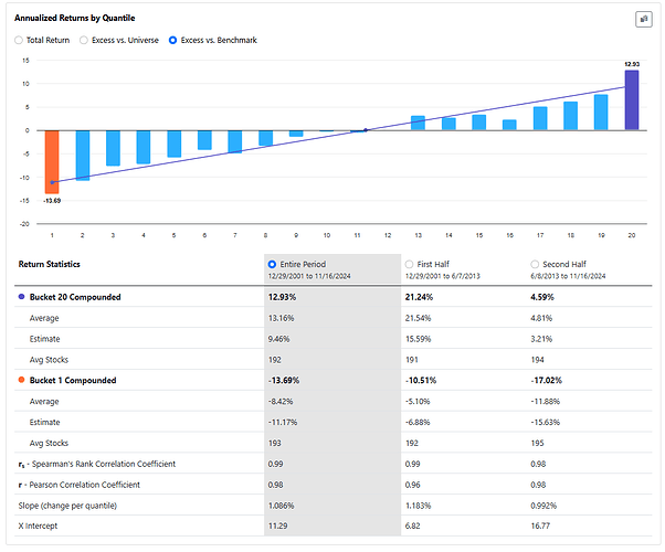
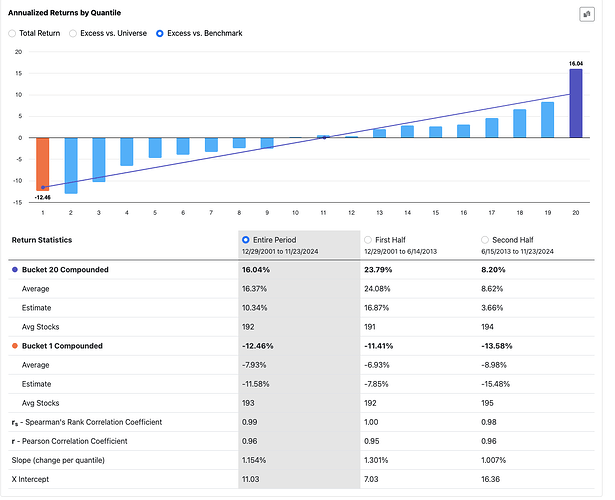
The Core Combination incl. Size ranking system on the Universe Easy to Trade US, with NA's neutral, will give these results.

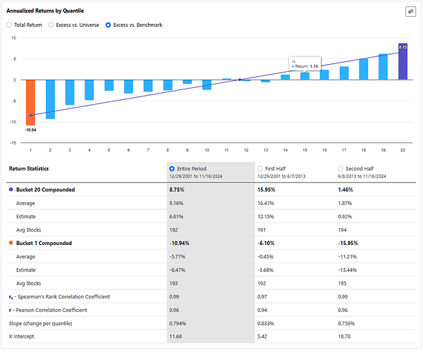
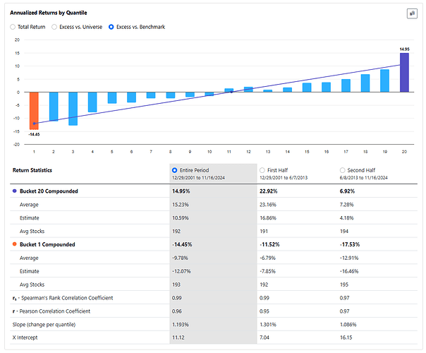
If you go through the process I described earlier and add universes, aggregate series and formulas for each factor and then run the factor timing ranking system on the Universe Easy to Trade US, with NA's neutral, you will find the following.

In case you run it with positive ánd negative weight adjustments with factor timing ranking system that allows for negative weights, you get:

.

In both cases, the results are worse than the original ranking system. I get similar results when I do this for my own ranking systems.

I really wish factor momentum would work, but it seems it does not. Am I missing something fundamental? If you’ve found success with factor momentum—or if you’ve struggled with similar results—I’d love to hear your thoughts.

Best,

Victor

[Jrinne]

@Victor1991

Am I missing something fundamental? If you’ve found success with factor momentum—or if you’ve struggled with similar results—I’d love to hear your thoughts.

Can't you test recent momentum of your factors by doing a sliding window for any ML model of your choosing with the sliding window being the period for which you expect a trend? I am suggesting that if there is a persistent trend the model will find that trend in the training (sliding window) and you can determine whether capturing any trend in the training data is beneficial in the validation or test data.

You can even do a grid-search with Python to find the optimal window size for capturing any trend.

Compare that to an expanding window and see if there is an improvement. The expanding window serving as a control.

I do think return data over short periods is noisy and you might want to use a method that has regularization such as ridge regression. But you can use regularization with LightGBM and other methods too.

People have different experiences with sliding vs expanding windows. Maybe due to differences in the factors used.

I tend to find better results with an expanding window myself. I use expanding windows in all of my funded models. Maybe I just have not tried the optimal window size yet but my results suggest the possibility that with your factors you are not missing anything fundamental. That maybe the factors you use do not trend reliably or that any trending for your factors does not have a large effect.

Or that any trending for some factors is countered by mean- reversion of other factors in my case.

[rwbattyaz]

When I see data that shows the opposite of what I predicted, I wonder if I should take an opposite stance. Have you considered under weighting the identified factors? You may be identifying them as they are about to mean revert.

In terms of factor momentum, I accept that it exists and explicitly detecting it to use it is difficult at best. Instead I have multiple systems using a diversity of factors and an external money management process to weight and even defund systems based on relative performance.

Cheers,
Rich

[Jrinne]

@Victor1991

I really wish factor momentum would work help me show that it actually does

It tried but...

Trending versus Mean Reversion in Factor Returns: A Technical Analysis

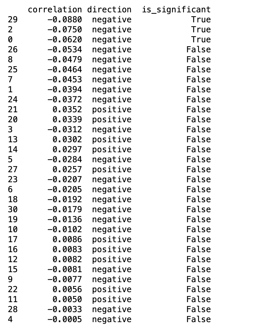
I analyzed the weekly returns of the top bucket for 31 different stock market factors to investigate their predictive properties. The key finding: weak predictive relationships (three statistically significant) with mean reversion dominating. NOTE: you would expect a few statistically positive tests of 31 factors, with multiple window sizes tested, by chance alone.

Methodology:

• Tested if the SMA over a period predicts average returns over the next 4 weeks
• Grid search for optimal SMA window sizes: [4, 8, 12, 16, 20, 24, 28, 32 weeks]
• Used linear regression to test predictive power
• Analyzed correlations, p-values, and statistical significance

Key Findings:

1. Evidence of weak predictive relationships:

   • Correlations range from -0.0880 to +0.0339
   • Three factors show statistical significance (p < 0.05)
   • 21 of 31 factors show negative correlations (mean-reverting tendency)
   • All best performing windows were 4 weeks

2. Window Size Analysis:

   • 4-week window emerged as optimal for all factors
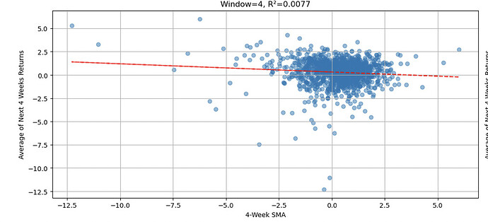
   • R-squared values all below 1%
   • Predominantly negative correlations suggesting mean reversion

Results table (name of factors removed):

Most significant regression results:

Code included for transparency and replication.

import pandas as pd
import numpy as np
from scipy import stats
import statsmodels.api as sm
import matplotlib.pyplot as plt
import seaborn as sns

def analyze_predictive_power(data_series, window):
    """
    Analyze predictive power of SMA for average of next 4 weeks' returns
    """
    # Calculate SMA
    sma = data_series.rolling(window=window).mean()
    
    # Calculate average return over next 4 weeks
    forward_returns = pd.concat([data_series.shift(-i) for i in range(1, 5)], axis=1).mean(axis=1)
    
    # Remove NAs from both series
    sma = sma[window:-4]  # Remove first window periods and last 4 periods
    forward_returns = forward_returns[window:-4]  # Align with SMA
    
    # Run regression of forward returns on SMA
    slope, intercept, r_value, p_value, std_err = stats.linregress(sma, forward_returns)
    
    # Calculate correlation
    correlation = sma.corr(forward_returns)
    
    return {
        'window': window,
        'slope': slope,
        'p_value': p_value,
        'r_squared': r_value**2,
        'correlation': correlation,
        'std_err': std_err,
        'direction': 'positive' if slope > 0 else 'negative',
        'is_significant': p_value < 0.05
    }

def analyze_all_metrics(data, windows=[4, 8, 12, 16, 20, 24, 28, 32]):
    """
    Analyze predictive power for all metrics
    """
    all_results = {}
    significant_predictions = []
    
    # Analyze each column
    for column in data.columns:
        if column != 'date':
            print(f"\nAnalyzing {column}...")
            
            # Test each window size
            window_results = []
            for window in windows:
                result = analyze_predictive_power(data[column], window)
                window_results.append(result)
            
            # Convert results to DataFrame
            results_df = pd.DataFrame(window_results)
            all_results[column] = results_df
            
            # Track significant predictions
            best_window = results_df.loc[results_df['r_squared'].idxmax()]
            if best_window['is_significant']:
                significant_predictions.append({
                    'metric': column,
                    'window': int(best_window['window']),
                    'r_squared': best_window['r_squared'],
                    'direction': best_window['direction'],
                    'p_value': best_window['p_value'],
                    'correlation': best_window['correlation']
                })
    
    return all_results, significant_predictions

# Read and prepare data
file_path = "insert_your_path"  # Replace with your file path
data = pd.read_csv(file_path)
data['date'] = pd.to_datetime(data['date'], format='%m/%d/%y')
data = data.set_index('date')

# Perform analysis
all_results, significant_predictions = analyze_all_metrics(data)

# Create summary of best windows for each metric
summary_data = []
for metric, results in all_results.items():
    best_result = results.loc[results_df['r_squared'].idxmax()]
    summary_data.append({
        'metric': metric,
        'best_window': int(best_result['window']),
        'r_squared': best_result['r_squared'],
        'p_value': best_result['p_value'],
        'correlation': best_result['correlation'],
        'direction': best_result['direction'],
        'is_significant': best_result['is_significant']
    })

summary_df = pd.DataFrame(summary_data)
summary_df = summary_df.sort_values('r_squared', ascending=False)

# Print summary results
print("\n=== Summary of Predictive Power Analysis ===")
pd.set_option('display.max_rows', None)
pd.set_option('display.float_format', lambda x: '%.4f' % x)
print(summary_df)

# Create visualization of top metrics
plt.figure(figsize=(20, 15))

# Select top 6 metrics by R-squared for visualization
top_metrics = list(summary_df.head(6)['metric'])

for i, metric in enumerate(top_metrics, 1):
    plt.subplot(3, 2, i)
    
    # Get best window for this metric
    best_window = int(summary_df[summary_df['metric'] == metric]['best_window'].values[0])
    
    # Calculate SMA and forward returns
    sma = data[metric].rolling(window=best_window).mean()
    forward_returns = pd.concat([data[metric].shift(-i) for i in range(1, 5)], axis=1).mean(axis=1)
    
    # Remove NAs
    sma = sma[best_window:-4]
    forward_returns = forward_returns[best_window:-4]
    
    # Create scatter plot
    plt.scatter(sma, forward_returns, alpha=0.5)
    
    # Add regression line
    z = np.polyfit(sma, forward_returns, 1)
    p = np.poly1d(z)
    plt.plot(sma, p(sma), "r--", alpha=0.8)
    
    plt.title(f'{metric}\nWindow={best_window}, R²={summary_df[summary_df["metric"]==metric]["r_squared"].values[0]:.4f}')
    plt.xlabel(f'{best_window}-Week SMA')
    plt.ylabel('Average of Next 4 Weeks Returns')
    plt.grid(True)

plt.tight_layout()
plt.show()

# Print key insights
print("\n=== Key Insights ===")
print(f"1. Total metrics analyzed: {len(summary_df)}")
print(f"2. Metrics with significant predictive power: {len(significant_predictions)}")
print("\n3. Top 5 most predictive metrics:")
print(summary_df.head().to_string())

# Additional analysis of significant predictors
if significant_predictions:
    print("\n4. Metrics with significant predictive power:")
    sig_df = pd.DataFrame(significant_predictions).sort_values('r_squared', ascending=False)
    print(sig_df.to_string())
else:
    print("\n4. No metrics showed significant predictive power")

# Create correlation heatmap for top metrics
top_10_metrics = summary_df.head(10)['metric'].tolist()
corr_matrix = data[top_10_metrics].corr()

plt.figure(figsize=(12, 10))
sns.heatmap(corr_matrix, annot=True, cmap='coolwarm', center=0)
plt.title('Correlation Matrix of Top 10 Predictive Metrics')
plt.tight_layout()
plt.show()

# Save results
summary_df.to_csv('predictive_power_analysis.csv')
if significant_predictions:
    pd.DataFrame(significant_predictions).to_csv('significant_predictors.csv')

[Victor1991]

@rwbattyaz

Have you considered under weighting the identified factors? You may be identifying them as they are about to mean revert.

Interestingly enough, treating it as a mean reversion seems to at least slighly improve results for most of my ranking systems. Especially if I do not give it too much weight. Just another sprinkle on top basically. I will experiment with it a bit more though before incorporating it. It could be the timeframe that I tested on (50 days), but it could also be something else.

[Victor1991]

Hi Jim,

Could you share what type of factors you have been using here? Was it a mix of the factor groups that I mentioned before (as defined in the Core combination ranking system) or mostly factors of a single type?

Reason I am asking is that I thought of the hypothesis that perhaps only factors of a certain type tend to trend and/or mean revert over these shorter timeframes.

[Jrinne]

@Victor1991

factors of a single type?

These were single factors that you would recognize with a lot being from the core ranking system. I would have done groups to duplicate what you have done--which is a good idea--but the spreadsheet I used was on my desktop just waiting to be used.

@Victor1991

the hypothesis that perhaps only factors of a certain type tend to trend and/or mean revert over these shorter timeframes.

Great question. I prefer not to discuss the particular features I use or how I select them. But generally I can say the factors that trended (rather than being mean reverting) were value factors and analyst revisions.

Great point about different factor types behaving differently and thanks for bringing it to my attention!

If the output is interesting, It should be easy to test the nodes or individual factors you are interested in with the code. It would be easy to change the grid search parameters and the target period. The csv file I uploaded in the code was just the download of the top bucket returns with the name of the factor as the heading—testing multiple factors or column headings at once. The code removes the date column from the csv file. It should run on most computers. Quickly I believe.

[yuvaltaylor]

@Victor1991

Using this approach, the better a factor group performs relative to other factors groups over a 50-day period, the higher the weight that factor group will have in the ranking system for that factor group in that week. The worst factor group will not get a higher weight.

Why a 50-day period? Stock momentum and industry momentum both work best over a six- to twelve-month period. With stock momentum you don't look at the most recent month. Would you get the same results with a 270-day period (calendar days) or a 200-bar period? Or a 270-day period ignoring the most recent month?

Also, there's an easier way to backtest this: go long the best two performing factors and short the worst two, just using your aggregate series. That won't tell you if factor momentum is something you can actually use, but it'll tell you if it exists.

[ZGWZ]

The (unique) effect of factor momentum is mainly in one month. This is why its basically useless.

[Jrinne]

Edit: Just to put this into perspective, I used my KNN method on 31 factors and compared each to 100 randomized models. No randomized model beat my model with the any of the target factors used. Suggesting a p-value < 0.0003 for the KNN model I am using having some predictive power. Maybe just me but no small thing, I think.

You could also assume there is a 50/50 chance that my method would work with any single factor. Then there would be a one in 2^31 chance that my model would work for every factor tried. Or you would expect that result occur 1 in 2,147,483,648 times by chance alone (with no predictive power for the model). It's like getting heads 31 times in a row with a fair coin by chance alone to use another non-parametric statistical method, if you like statistics but question the first method.

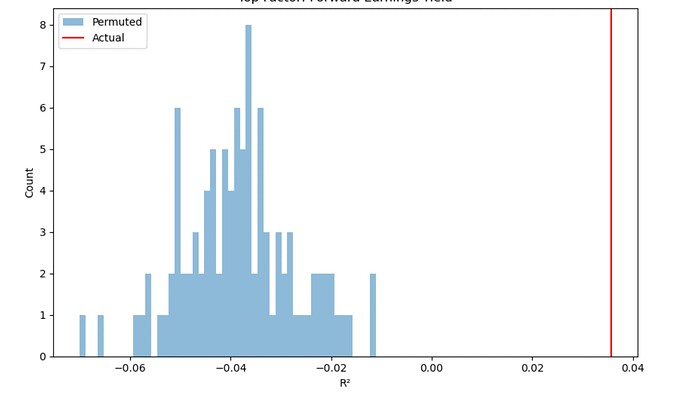
For a visualization of this method here is the permuted or randomized results compared to the actual results of one facto. The permutations could be normally distributed. If so about a 3 sigma event for just one factor I would say just eyeballing the results:

TL;DR: I agree with everyone's post above. But maybe whom I agree with depends on the feature and the period. And I wonder why I would have to rely on just one piece of data (or one predictor). Why would I do that?

My opinion based on some data (see above) is that all of the above can be true depending on the feature and period used. That you can have momentum or mean reversion and that it may or may not be a large effect and may or may not be statistically significant

Yuval adds that is it possible to see momentum over longer periods but mean-reversion over shorter periods. True for sure and this is commonly used in the literature which supports his idea. An important contribution to this discussion, I believe.

Why assume a priori it will be one or the other. And if there is momentum over the longer period but mean reversion over the shorter period why not include both in your predictive model?

Do you assume all factors will behave the same over all periods? If not, what model do you use to begin to discriminate among features? Whatever you decide to do will you want to do the same thing for every feature?

So whatever one believes about a particular factor how do you use what you believe? And if you are going to use a model which one will you use? I used linear regression above and I think that works pretty good if you are going to use just one piece of data for predictions. But there are other ways to do it.

What if you wanted to use the idea that there is a trend long-term but mean reversion short term? MAYBE YOU BELIEVE THERE IS AN INTERACTION BETWEEN THESE 2 FEATURES. And maybe some other data too? Maybe there is macro data that is correlsted with you factor's performance (like interest rate changes) and you want to incorporate that?

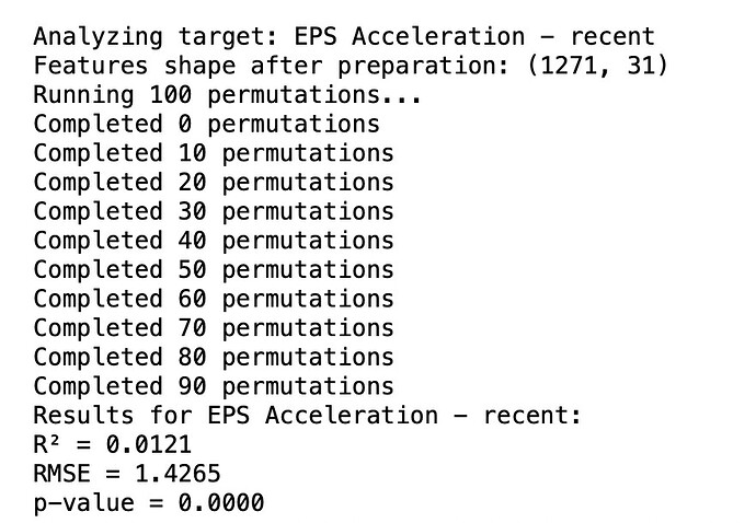
What model do you use for any of that. Here is how K-nearest neighbors (KNN) does with one target feature in the Core Ranking System and importantly multple predictors:

P-value is done in a unique way. The model is run with all of the factors I decided to use and a R^2 value obtained. Then the model was run multiple times with all of the features shuffled as is done here in Sklearn: Permutation feature importance. In this example there were 100 runs with the features shuffled (reshuffled with each run) and none of them beat the model with real data suggesting the data was helpful for making predictions 100 times out of 100 runs..

If you have more time you can use more permutations. And before you fund it you could consider using Permutation feature importance to help you decide which features have the most predictive power and maybe remove a few features that seem to be just noise.

@ZGWZ

The (unique) effect of factor momentum is mainly in one month. This is why it's basically useless.

My grid search of a relatively small amount of data would confirm 4 weeks has a strong effect if you are considering both mean reversion and trending.. The above KNN model uses 4 weeks for the predictors for that reason. Confirmation of what you have said, I believe.

BTW, I am finding statistical significance (as determined by the feature permutation method above) for every feature I have tested with KNN so far. Suggesting everyone's ideas can be incorporated into one objective model using multiple features to do so. It would not have to be KNN but I have a fondness for it as it's actually the simplest ML model, does not assume the data is normally distributed, uses interactions for predictions and, when keeping the number of features small, hard to beat.

JIm

[Victor1991]

@yuvaltaylor

Why a 50-day period?

I read literature where it was mentioned that for factor momentum, persistence mainly occurs when using short lookback periods. I'm assuming that's why ZGWZ also mentions this.

@ZGWZ

The (unique) effect of factor momentum is mainly in one month. This is why its basically useless.

I've tried out some different lookback periods today, using the same methodology that I described earlier. Basically across most lookback periods mean-reversion (so basically inverting the node) worked better for me than betting on momentum. Also, the further I went down the timeline (starting at 20-day and after 50-day, 100-day, 200-day ending at 250-day), the stronger the mean reversion results became. From my understanding now, I would do better going for a 20 minus 250 day factor momentum strategy (i.e. a mean reversion approach), than the opposite way around.

See below for the results (20 day returns - 250 day returns) applied to the Core Combination ranking system, with the factor reversion having 10/110% weight.

@yuvaltaylor

Also, there's an easier way to backtest this: go long the best two performing factors and short the worst two, just using your aggregate series.

Would you want to elaborate on how to do this in P123? I'm assuming with a screen, but the exact way to do it, I do not see right away. It would probably save me a lot of time when researching this topic.

[yuvaltaylor]

@Victor1991

Would you want to elaborate on how to do this in P123? I'm assuming with a screen, but the exact way to do it, I do not see right away. It would probably save me a lot of time when researching this topic.

Off the top of my head, you'd create variables in a screen for all the aggregate series using Close(0,[name of series]). Then you'd write rules that get at the maximum and minimum of those series. Lastly, you'd apply your universe rules accordingly on the long and short sides of the screen.

Does that make sense? Maybe it's more complicated than your method, in which case I was mistaken when I said it was easier.

[yuvaltaylor]

Thanks. That's a very good point indeed. I forgot that this was the case in the academic literature, and I apologize for questioning the 50-day period.