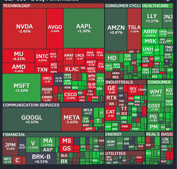
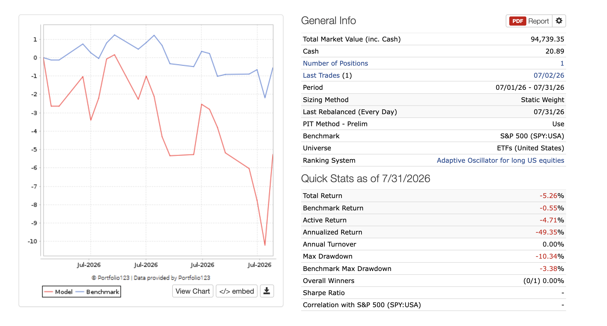
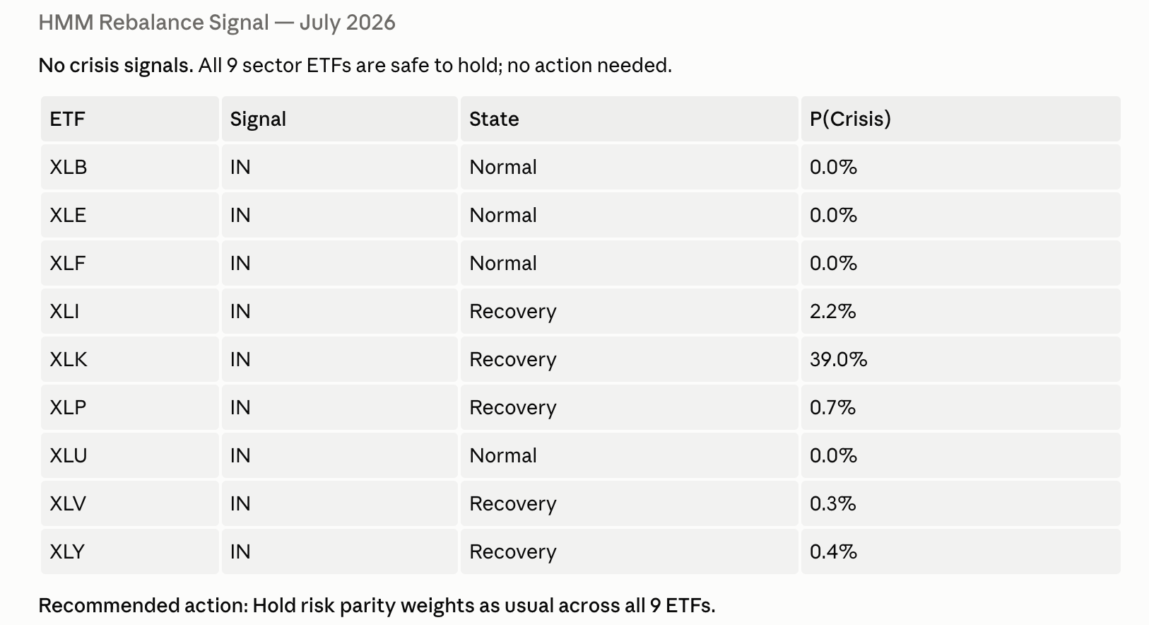
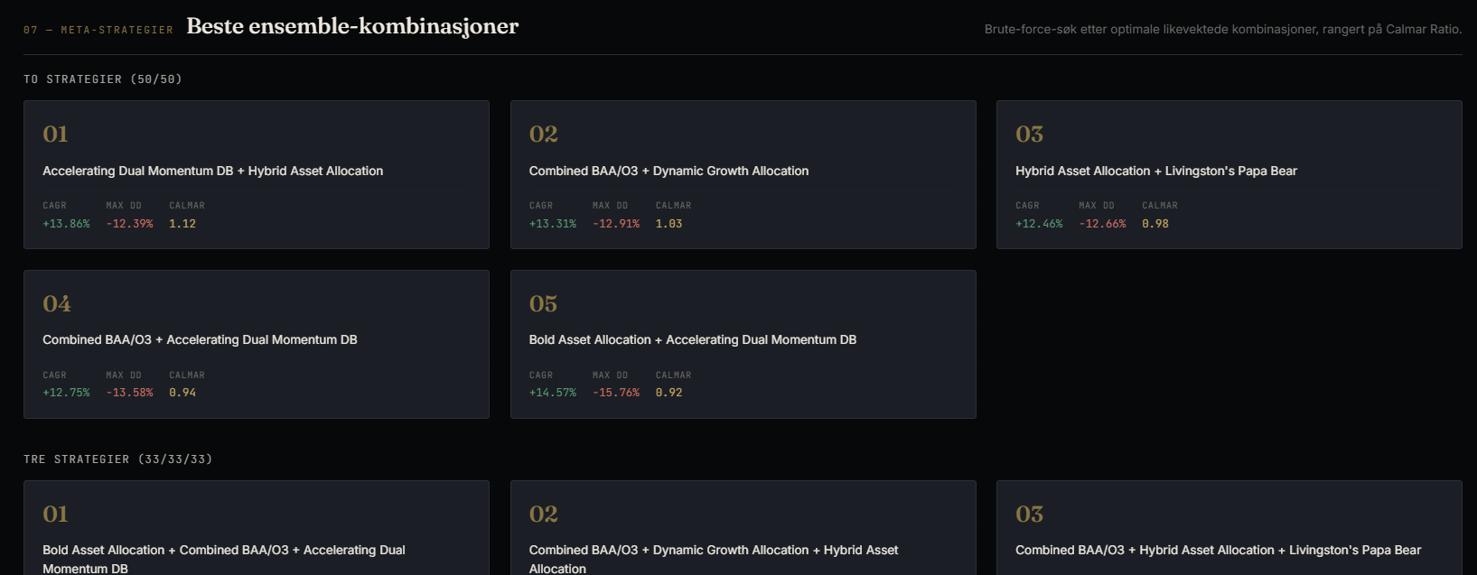
I don't know if it's true, and I know that timing the market doesn't work, but I still have a feeling that a correction might be approaching. I have tried various solutions for hedging, ranging from using alternative strategies on AllocateSmartly (which I have now developed my own scripts to adapt to some ideas from that site) to an attempt at implementing Yuval T's put strategy (I have attached the script I used).
But does anyone have success with good yet inexpensive hedging strategies? Does anyone use, for example, Short ETF solutions for effective hedging, or other approaches?
# -*- coding: utf-8 -*-
"""

"""

import datetime as dt
import pandas as pd
import yfinance as yf
import numpy as np
from scipy.stats import norm, percentileofscore
from concurrent.futures import ThreadPoolExecutor
import logging
import time
from pathlib import Path

# ============================================================================
# KONFIGURASJON - JUSTER DISSE ETTER BEHOV
# ============================================================================

# Taylor-spesifikke parametre
TAYLOR_BS_DISCOUNT = 0.60           # Taylor betaler typisk 40-60% av B-S pris (justert opp)
MAX_IV_RANK = 70                    # Kjøp kun når IV rank < 70 (mer fleksibelt)
MIN_EXPECTED_ANNUAL_RETURN = 0.30   # Minimum 30% forventet årlig avkastning (mer realistisk)

# Tidsramme (fra artikkel)
MIN_EXP_MONTHS = 3                  # Minimum 3 måneder (Taylor: >2-3 mnd)
MAX_EXP_MONTHS = 9                  # Maksimum 9 måneder (Taylor: <9 mnd)

# Likviditet (lavere krav - Taylor bruker GTC orders uansett)
MIN_OPEN_INTEREST = 1               # Minimum 1 (kan bruke GTC orders)
MIN_VOLUME = 0                      # Ingen volum-krav (GTC orders)

# Performance
MAX_WORKERS = 2
SLEEP_TIME = 1.5
RISK_FREE_RATE = 0.045              # Oppdatert risikofri rente (4.5%)

# Output - KUN terminal, ingen CSV
DISPLAY_TOP_N = 50  # Hvor mange opsjoner å vise

# ============================================================================
# LOGGING
# ============================================================================

logging.basicConfig(
    level=logging.INFO,
    format='%(asctime)s - %(levelname)s - %(message)s'
)

# ============================================================================
# HJELPEFUNKSJONER
# ============================================================================

def parse_scores(score_str):
    """Parser ticker + score string til dictionary"""
    scores = {}
    for line in score_str.strip().split('\n'):
        try:
            parts = line.split()
            if len(parts) >= 2:
                ticker = parts[0].strip()
                score = float(parts[-1])
                scores[ticker] = score
        except (ValueError, Exception) as e:
            logging.warning(f"Kunne ikke parse: '{line}' - {e}")
    return scores


def normalize_scores(scores):
    """Normaliser scores (0-1), høyere = dårligere aksje"""
    if not scores:
        return {}

    valid = {k: v for k, v in scores.items() if pd.notna(v)}
    if not valid:
        return {t: 0.5 for t in scores}

    max_s = max(valid.values())
    min_s = min(valid.values())

    if max_s == min_s:
        return {t: 0.5 for t in scores}

    return {
        t: (s - min_s) / (max_s - min_s) if pd.notna(s) else np.nan
        for t, s in scores.items()
    }


def filter_expirations(expirations, min_months=MIN_EXP_MONTHS, max_months=MAX_EXP_MONTHS):
    """Filtrer utløpsdatoer (3-9 måneder)"""
    now = dt.datetime.now()
    min_date = now + dt.timedelta(days=30 * min_months)
    max_date = now + dt.timedelta(days=30 * max_months)

    filtered = []
    for exp_str in expirations:
        try:
            exp_date = dt.datetime.strptime(exp_str, "%Y-%m-%d")
            if min_date <= exp_date <= max_date:
                filtered.append(exp_str)
        except ValueError:
            continue

    logging.debug(f"Filtrerte utløp: {len(filtered)} datoer mellom {min_months}-{max_months} mnd")
    return filtered


def calculate_historical_volatility(symbol, window='1y'):
    """Beregner annualisert historisk volatilitet"""
    try:
        tk = yf.Ticker(symbol)
        hist = tk.history(period=window)

        if hist.empty or len(hist) < 10:
            return np.nan

        hist['LogReturn'] = np.log(hist['Close'] / hist['Close'].shift(1))
        hist = hist.dropna(subset=['LogReturn'])

        if len(hist) < 10:
            return np.nan

        # Annualisert volatilitet (i desimaler, ikke prosent)
        vol = hist['LogReturn'].std() * np.sqrt(252)
        return vol

    except Exception as e:
        logging.error(f"Feil ved HV for {symbol}: {e}")
        return np.nan


def calculate_iv_rank(current_iv, historical_vol_1y, historical_vol_6m):
    """
    Beregner IV Rank - hvor billig er opsjonen?

    Taylor kjøper når IV er LAV (billige opsjoner)
    IV Rank < 30 = Veldig billig
    IV Rank < 50 = Rimelig
    IV Rank > 60 = For dyrt
    """
    if pd.isna(current_iv) or pd.isna(historical_vol_1y):
        return np.nan

    # Sammenlign med historisk volatilitet
    # Hvis IV << HV, er opsjonene billige
    avg_hv = np.nanmean([historical_vol_1y, historical_vol_6m])

    if pd.isna(avg_hv) or avg_hv <= 0:
        return np.nan

    # IV Rank: hvor er IV relativt til HV? (0-100 skala)
    iv_rank = (current_iv / avg_hv) * 50  # Skalert til ~0-100

    return min(100, max(0, iv_rank))


def calculate_black_scholes_put(S, K, T, r, sigma):
    """Black-Scholes Put pris"""
    if any(pd.isna([S, K, T, r, sigma])) or sigma <= 1e-6 or T <= 1e-6:
        return np.nan

    try:
        d1 = (np.log(S / K) + (r + 0.5 * sigma**2) * T) / (sigma * np.sqrt(T))
        d2 = d1 - sigma * np.sqrt(T)

        put_price = K * np.exp(-r * T) * norm.cdf(-d2) - S * norm.cdf(-d1)
        return max(0.0, put_price)

    except Exception as e:
        logging.debug(f"B-S feil: {e}")
        return max(0.0, K - S) if pd.notna(K) and pd.notna(S) else np.nan


def calculate_taylor_metrics(row, score, normalized_score, hv_1y, hv_6m):
    """
    Beregner Taylor-spesifikke metrikker for én opsjon

    Returns: dict med alle nødvendige verdier
    """
    metrics = {}

    # Basis verdier
    S = row['stockPrice']
    K = row['strike']
    T = row['timeToMaturity']
    r = RISK_FREE_RATE
    IV = row['impliedVolatility'] / 100 if pd.notna(row['impliedVolatility']) else np.nan
    last_price = row['lastPrice']

    # 1. Black-Scholes pris med historisk volatilitet
    if pd.notna(hv_6m) and hv_6m > 0:
        bs_hv_price = calculate_black_scholes_put(S, K, T, r, hv_6m)
    else:
        bs_hv_price = np.nan

    metrics['bs_hv_price'] = bs_hv_price

    # 2. Taylor Max Price: Typisk 40-50% av B-S, justert for score
    #    Høyere score (dårligere aksje) = kan betale litt mer
    if pd.notna(bs_hv_price) and bs_hv_price > 0:
        # Base discount
        discount = TAYLOR_BS_DISCOUNT

        # Juster for score (normalisert 0-1)
        # Høyere normalized_score = dårligere aksje = litt høyere max pris
        score_adjustment = 1 + (normalized_score * 0.3)  # 1.0 til 1.3

        taylor_max = bs_hv_price * discount * score_adjustment
        metrics['taylor_max_price'] = taylor_max

        # Hvor billig er opsjonen vs. Taylors maks?
        if last_price > 0:
            metrics['price_vs_taylor_max'] = last_price / taylor_max
        else:
            metrics['price_vs_taylor_max'] = np.nan
    else:
        metrics['taylor_max_price'] = np.nan
        metrics['price_vs_taylor_max'] = np.nan

    # 3. IV Rank
    metrics['iv_rank'] = calculate_iv_rank(IV, hv_1y, hv_6m)

    # 4. Expected Return (forenklet)
    #    Antar at aksjen kan falle med 20-40% (basert på score)
    #    Høyere score = større forventet fall
    if pd.notna(last_price) and last_price > 0 and pd.notna(S) and pd.notna(K):
        # Forventet prisfall basert på score
        expected_drop_pct = 0.15 + (normalized_score * 0.25)  # 15% til 40%
        expected_price = S * (1 - expected_drop_pct)

        # Forventet payoff
        expected_payoff = max(0, K - expected_price)
        expected_profit = expected_payoff - last_price

        if expected_profit > 0:
            expected_return = expected_profit / last_price
            # Annualisert
            if T > 0:
                expected_annual_return = (1 + expected_return) ** (1/T) - 1
            else:
                expected_annual_return = np.nan
        else:
            expected_return = -1
            expected_annual_return = -1

        metrics['expected_return'] = expected_return
        metrics['expected_annual_return'] = expected_annual_return
    else:
        metrics['expected_return'] = np.nan
        metrics['expected_annual_return'] = np.nan

    # 5. Break-even pris
    if pd.notna(K) and pd.notna(last_price):
        metrics['breakeven_price'] = K - last_price
        if pd.notna(S) and S > 0:
            metrics['breakeven_drop_pct'] = (S - metrics['breakeven_price']) / S
        else:
            metrics['breakeven_drop_pct'] = np.nan
    else:
        metrics['breakeven_price'] = np.nan
        metrics['breakeven_drop_pct'] = np.nan

    return metrics


def process_ticker(symbol, score, normalized_score, risk_free_rate, sleep_time):
    """
    Hovedfunksjon: Analyser én ticker og finn beste put-opsjoner

    Følger Taylors prinsipper:
    1. OTM puts, 3-9 måneder
    2. Kun når IV er lav (billige opsjoner)
    3. Må være billigere enn Taylor max price
    4. Forventet avkastning må være høy nok
    """
    logging.debug(f"Venter {sleep_time:.1f}s før {symbol}...")
    time.sleep(sleep_time)

    try:
        logging.info(f"=== Analyserer {symbol} (Score: {score:.2f}) ===")
        tk = yf.Ticker(symbol)

        # 1. Hent aksjekurs
        try:
            hist = tk.history(period="1d")
            if hist.empty or 'Close' not in hist.columns:
                logging.warning(f"Ingen kurs for {symbol}")
                return pd.DataFrame()

            current_price = hist['Close'].iloc[-1]
            if pd.isna(current_price):
                logging.warning(f"Kurs er NaN for {symbol}")
                return pd.DataFrame()

            logging.info(f"Kurs: ${current_price:.2f}")

        except Exception as e:
            logging.error(f"Feil ved henting av kurs for {symbol}: {e}")
            return pd.DataFrame()

        # 2. Beregn historisk volatilitet (1 år og 6 mnd)
        hv_1y = calculate_historical_volatility(symbol, window='1y')
        hv_6m = calculate_historical_volatility(symbol, window='6mo')

        if pd.isna(hv_6m):
            logging.warning(f"Kunne ikke beregne HV for {symbol}")
            return pd.DataFrame()

        logging.info(f"HV 6m: {hv_6m*100:.1f}%, HV 1y: {hv_1y*100:.1f}%")

        # 3. Hent opsjonsdata
        try:
            expirations = tk.options
            if not expirations:
                logging.warning(f"Ingen opsjoner for {symbol}")
                return pd.DataFrame()
        except Exception as e:
            logging.error(f"Feil ved henting av opsjoner for {symbol}: {e}")
            return pd.DataFrame()

        filtered_exp = filter_expirations(expirations)
        if not filtered_exp:
            logging.warning(f"Ingen utløpsdatoer {MIN_EXP_MONTHS}-{MAX_EXP_MONTHS} mnd for {symbol}")
            return pd.DataFrame()

        # 4. Samle puts fra alle utløpsdatoer
        all_puts = []
        for exp_date in filtered_exp:
            try:
                time.sleep(sleep_time / 4)
                options = tk.option_chain(exp_date)
                puts = options.puts

                if puts is not None and not puts.empty:
                    puts['expirationDate'] = pd.to_datetime(exp_date)
                    all_puts.append(puts)

            except Exception as e:
                logging.error(f"Feil ved henting av puts for {symbol} ({exp_date}): {e}")
                continue

        if not all_puts:
            logging.warning(f"Ingen puts funnet for {symbol}")
            return pd.DataFrame()

        data = pd.concat(all_puts, ignore_index=True)

        # 5. Filtrer OTM puts
        otm_puts = data[data['strike'] < current_price * 0.995].copy()

        if otm_puts.empty:
            logging.info(f"Ingen OTM puts for {symbol}")
            return pd.DataFrame()

        logging.info(f"Fant {len(otm_puts)} OTM puts")

        # 6. Legg til basisinfo
        otm_puts['underlyingSymbol'] = symbol
        otm_puts['stockPrice'] = current_price
        otm_puts['originalScore'] = score
        otm_puts['normalizedScore'] = normalized_score

        # 7. Beregn tid til utløp
        now_dt = pd.Timestamp.now(tz='UTC')
        if otm_puts['expirationDate'].dt.tz is None:
            otm_puts['expirationDate'] = otm_puts['expirationDate'].dt.tz_localize('UTC')

        exp_dt = otm_puts['expirationDate'] + pd.Timedelta(hours=16)
        otm_puts['timeToMaturity'] = (exp_dt - now_dt).dt.total_seconds() / (365.25 * 24 * 3600)
        otm_puts = otm_puts[otm_puts['timeToMaturity'] > 0.01]

        if otm_puts.empty:
            return pd.DataFrame()

        # 8. Sikre numeriske verdier
        otm_puts['strike'] = pd.to_numeric(otm_puts['strike'], errors='coerce')
        otm_puts['lastPrice'] = pd.to_numeric(otm_puts['lastPrice'], errors='coerce')
        otm_puts['bid'] = pd.to_numeric(otm_puts['bid'], errors='coerce')
        otm_puts['ask'] = pd.to_numeric(otm_puts['ask'], errors='coerce')
        otm_puts['volume'] = pd.to_numeric(otm_puts['volume'], errors='coerce').fillna(0)
        otm_puts['openInterest'] = pd.to_numeric(otm_puts['openInterest'], errors='coerce').fillna(0)
        otm_puts['impliedVolatility'] = pd.to_numeric(otm_puts['impliedVolatility'], errors='coerce') * 100

        # 9. Filtrer på likviditet
        initial_count = len(otm_puts)
        otm_puts = otm_puts[
            (otm_puts['openInterest'] >= MIN_OPEN_INTEREST) |
            (otm_puts['volume'] >= MIN_VOLUME)
        ]
        logging.info(f"Etter likviditetsfilter: {len(otm_puts)}/{initial_count}")

        if otm_puts.empty:
            return pd.DataFrame()

        # 10. TAYLOR-ANALYSE: Beregn alle metrikker
        taylor_metrics_list = []
        for idx, row in otm_puts.iterrows():
            metrics = calculate_taylor_metrics(row, score, normalized_score, hv_1y, hv_6m)
            taylor_metrics_list.append(metrics)

        # Legg til som nye kolonner
        metrics_df = pd.DataFrame(taylor_metrics_list)
        otm_puts = pd.concat([otm_puts.reset_index(drop=True), metrics_df], axis=1)

        # 11. TAYLOR FILTRE

        # Filter 1: IV Rank (kun advarsel, ikke hard filter)
        valid_iv = otm_puts['iv_rank'].notna()
        if valid_iv.any():
            high_iv_count = (otm_puts['iv_rank'] > MAX_IV_RANK).sum()
            if high_iv_count > 0:
                logging.info(f"⚠️  {high_iv_count} opsjoner har høy IV rank (>{MAX_IV_RANK}) - vær forsiktig")
            # IKKE filtrer bort - la bruker vurdere selv

        # Filter 2: Pris må være under Taylor max
        before = len(otm_puts)
        otm_puts = otm_puts[
            pd.notna(otm_puts['price_vs_taylor_max']) &
            (otm_puts['price_vs_taylor_max'] < 1.0)
        ]
        logging.info(f"Taylor max pris filter: {len(otm_puts)}/{before}")

        if otm_puts.empty:
            logging.info(f"Ingen opsjoner passerte Taylor-filtrene for {symbol}")
            return pd.DataFrame()

        # Filter 3: Forventet avkastning (advarsel, ikke hard filter)
        before = len(otm_puts)
        low_return = (
            pd.notna(otm_puts['expected_annual_return']) &
            (otm_puts['expected_annual_return'] < MIN_EXPECTED_ANNUAL_RETURN)
        ).sum()

        if low_return > 0:
            logging.info(f"⚠️  {low_return} opsjoner har lav forventet avkastning (<{MIN_EXPECTED_ANNUAL_RETURN*100:.0f}%)")

        # Behold alle, men merk de med lav avkastning
        otm_puts['meets_return_threshold'] = (
            otm_puts['expected_annual_return'] >= MIN_EXPECTED_ANNUAL_RETURN
        )

        if otm_puts.empty:
            logging.info(f"Ingen opsjoner passerte noen filtre for {symbol}")
            return pd.DataFrame()

        # 12. Beregn "Taylor Score" for rangering
        #     Kombinerer flere faktorer

        # Gi bonus til de som møter threshold
        return_bonus = otm_puts['meets_return_threshold'].astype(int) * 15

        otm_puts['taylor_score'] = (
            # Lavere pris vs max = bedre
            (1 - otm_puts['price_vs_taylor_max']) * 40 +

            # Lavere IV rank = bedre (hvis tilgjengelig)
            (1 - otm_puts['iv_rank'].fillna(50) / 100) * 25 +

            # Høyere forventet avkastning = bedre
            (otm_puts['expected_annual_return'].fillna(0).clip(upper=2.0) / 2.0) * 20 +

            # Høyere normalized score (dårligere aksje) = bedre
            otm_puts['normalizedScore'] * 10 +

            # Bonus for å møte return threshold
            return_bonus
        )

        # Legg til kvalitetsindikator
        otm_puts['quality'] = 'OK'
        otm_puts.loc[otm_puts['price_vs_taylor_max'] < 0.7, 'quality'] = 'GOOD'
        otm_puts.loc[
            (otm_puts['price_vs_taylor_max'] < 0.5) &
            (otm_puts['iv_rank'].fillna(100) < 40),
            'quality'
        ] = 'EXCELLENT'

        logging.info(f"✅ Fant {len(otm_puts)} kvalifiserte puts for {symbol}")
        return otm_puts

    except Exception as e:
        logging.exception(f"Uventet feil for {symbol}: {e}")
        return pd.DataFrame()


# ============================================================================
# HOVEDPROGRAM
# ============================================================================

def main(score_str):
    """
    Hovedfunksjon som kjører hele analysen
    """

    print("\n" + "="*80)
    print("TAYLOR PUT OPTIONS SCREENER")
    print("="*80)
    print(f"\n⚙️  KONFIGURASJON:")
    print(f"   • Tidsramme: {MIN_EXP_MONTHS}-{MAX_EXP_MONTHS} måneder")
    print(f"   • Max pris: {TAYLOR_BS_DISCOUNT*100:.0f}% av Black-Scholes")
    print(f"   • IV Rank advarselsgrense: {MAX_IV_RANK}")
    print(f"   • Min forventet avkastning (anbefalt): {MIN_EXPECTED_ANNUAL_RETURN*100:.0f}% årlig")
    print(f"   • Parallelle tråder: {MAX_WORKERS}")
    print(f"   • Viser: Topp {DISPLAY_TOP_N} opsjoner")
    print("\n" + "="*80 + "\n")

    # Parse scores
    scores = parse_scores(score_str)
    normalized_scores = normalize_scores(scores)
    tickers = list(scores.keys())

    logging.info(f"Antall tickere: {len(tickers)}")

    # Kjør analyse
    results = []
    with ThreadPoolExecutor(max_workers=MAX_WORKERS) as executor:
        tasks = []
        for symbol in tickers:
            if symbol in scores and symbol in normalized_scores:
                if pd.notna(scores[symbol]) and pd.notna(normalized_scores[symbol]):
                    tasks.append(
                        executor.submit(
                            process_ticker,
                            symbol,
                            scores[symbol],
                            normalized_scores[symbol],
                            RISK_FREE_RATE,
                            SLEEP_TIME
                        )
                    )

        logging.info(f"Sendt {len(tasks)} oppgaver til analyse...\n")

        for i, future in enumerate(tasks, 1):
            try:
                result = future.result()
                if result is not None and not result.empty:
                    results.append(result)

                if i % 10 == 0:
                    logging.info(f"Ferdig med {i}/{len(tasks)} tickere")

            except Exception as e:
                logging.error(f"Feil ved henting av resultat: {e}")

    # Analyser resultater
    if not results:
        print("\n⚠️  INGEN OPSJONER FUNNET")
        print("Mulige årsaker:")
        print("  • Markedet er for dyrt (høy IV)")
        print("  • Ingen opsjoner møter Taylors strenge kriterier")
        print("  • Prøv å øke TAYLOR_BS_DISCOUNT eller MAX_IV_RANK")
        return

    # Kombiner alle resultater
    all_puts = pd.concat(results, ignore_index=True)
    logging.info(f"\n✅ Totalt {len(all_puts)} opsjoner funnet på tvers av {len(results)} aksjer")

    # Sorter på Taylor Score
    all_puts = all_puts.sort_values('taylor_score', ascending=False)

    # Velg topp 3 per ticker (diversifisering)
    top_per_ticker = all_puts.groupby('underlyingSymbol').head(3)

    # Velg topp 30 totalt
    top_opportunities = all_puts.head(30)

    # ========================================================================
    # VISNING
    # ========================================================================

    display_cols = [
        'underlyingSymbol',
        'taylor_score',
        'quality',
        'originalScore',
        'contractSymbol',
        'lastPrice',
        'taylor_max_price',
        'price_vs_taylor_max',
        'strike',
        'stockPrice',
        'expirationDate',
        'timeToMaturity',
        'iv_rank',
        'expected_annual_return',
        'breakeven_price',
        'breakeven_drop_pct',
        'bid',
        'ask',
        'volume',
        'openInterest'
    ]

    display_cols = [c for c in display_cols if c in top_opportunities.columns]
    display_df = top_opportunities[display_cols].copy()

    # Formater datoer
    if 'expirationDate' in display_df:
        display_df['expirationDate'] = display_df['expirationDate'].dt.strftime('%Y-%m-%d')

    # Vis resultater
    print("\n" + "="*80)
    print(f"🎯 TOPP {DISPLAY_TOP_N} PUT-OPSJONER (Taylor-metoden)")
    print("="*80)
    print("\n📊 KOLONNE-FORKLARING:")
    print("  • CONTRACT: Fullt opsjonsnavn (bruk dette til å bestille)")
    print("  • T_SCORE: Taylor score (høyere = bedre kombinasjon av faktorer)")
    print("  • QUAL: Kvalitet (EXCELLENT/GOOD/OK basert på pris og IV)")
    print("  • F_SCORE: Din fundamental score (99.97 = verst aksje)")
    print("  • prc/max: Pris vs Taylor max (<0.5=SVÆRT billig, <0.8=Bra, <1.0=OK)")
    print("  • IV_RNK: IV rank (<30=Svært billig, <50=Billig, >60=Dyr)")
    print("  • exp_ret_%: Forventet årlig avkastning hvis aksjen faller som antatt")
    print("  • be_drop_%: Hvor mye må aksjen falle for break-even?")
    print("\n💡 Fokuser på: QUAL=EXCELLENT/GOOD + T_SCORE>60 + prc/max<0.8")
    print("-"*80 + "\n")

    # Vis alle resultater pent formatert
    pd.set_option('display.max_rows', None)
    pd.set_option('display.max_columns', None)
    pd.set_option('display.width', 250)  # Økt fra 200 for CONTRACT-kolonne
    pd.set_option('display.max_colwidth', 35)  # Max lengde for CONTRACT
    pd.set_option('display.float_format', '{:.2f}'.format)

    # Formater numeriske kolonner for bedre lesbarhet
    display_formatted = display_df.copy()

    # Prosentkolonner
    if 'expected_annual_return' in display_formatted:
        display_formatted['exp_ret_%'] = (display_formatted['expected_annual_return'] * 100).round(0).astype(int)
        display_formatted = display_formatted.drop('expected_annual_return', axis=1)

    if 'breakeven_drop_pct' in display_formatted:
        display_formatted['be_drop_%'] = (display_formatted['breakeven_drop_pct'] * 100).round(0).astype(int)
        display_formatted = display_formatted.drop('breakeven_drop_pct', axis=1)

    # Tid til utløp i dager
    if 'timeToMaturity' in display_formatted:
        display_formatted['days'] = (display_formatted['timeToMaturity'] * 365).round(0).astype(int)
        display_formatted = display_formatted.drop('timeToMaturity', axis=1)

    # Rund av scores
    for col in ['taylor_score', 'originalScore', 'iv_rank']:
        if col in display_formatted:
            display_formatted[col] = display_formatted[col].round(0).astype(int)

    # Rund av ratios til 2 desimaler
    if 'price_vs_taylor_max' in display_formatted:
        display_formatted['prc/max'] = display_formatted['price_vs_taylor_max'].round(2)
        display_formatted = display_formatted.drop('price_vs_taylor_max', axis=1)

    # Forenkle kolonnenavn
    rename_map = {
        'underlyingSymbol': 'TICKER',
        'taylor_score': 'T_SCORE',
        'quality': 'QUAL',
        'originalScore': 'F_SCORE',
        'contractSymbol': 'CONTRACT',
        'lastPrice': 'PRICE',
        'taylor_max_price': 'MAX_PRC',
        'strike': 'STRIKE',
        'stockPrice': 'STOCK',
        'expirationDate': 'EXPIRY',
        'iv_rank': 'IV_RNK',
        'breakeven_price': 'BREAKEVEN',
        'bid': 'BID',
        'ask': 'ASK',
        'volume': 'VOL',
        'openInterest': 'OI'
    }

    display_formatted = display_formatted.rename(columns=rename_map)

    # Velg kolonner i best rekkefølge
    priority_cols = [
        'TICKER', 'CONTRACT', 'T_SCORE', 'QUAL', 'F_SCORE', 'prc/max',
        'PRICE', 'MAX_PRC', 'STRIKE', 'STOCK', 'EXPIRY', 'days', 'IV_RNK',
        'exp_ret_%', 'be_drop_%', 'BREAKEVEN', 'BID', 'ASK', 'VOL', 'OI'
    ]

    final_cols = [c for c in priority_cols if c in display_formatted.columns]
    display_formatted = display_formatted[final_cols]

    print(display_formatted.to_string(index=False, max_rows=DISPLAY_TOP_N))

    # Oppsummering
    print("\n" + "="*80)
    print("📊 OPPSUMMERING")
    print("="*80)
    print(f"• Antall aksjer analysert: {len(tickers)}")
    print(f"• Aksjer med kvalifiserte opsjoner: {len(results)}")
    print(f"• Totalt kvalifiserte opsjoner: {len(all_puts)}")
    print(f"• Gjennomsnittlig Taylor Score: {all_puts['taylor_score'].mean():.1f}")
    print(f"• Gjennomsnittlig pris: ${all_puts['lastPrice'].mean():.2f}")
    print(f"• Gjennomsnittlig forventet årlig avkastning: {all_puts['expected_annual_return'].mean()*100:.1f}%")

    # Topp 5 aksjer
    top_stocks = (
        all_puts.groupby('underlyingSymbol')
        .agg({
            'taylor_score': 'max',
            'lastPrice': 'mean',
            'expected_annual_return': 'mean'
        })
        .sort_values('taylor_score', ascending=False)
        .head(5)
    )

    print("\n🏆 TOPP 5 AKSJER:")
    for symbol, row in top_stocks.iterrows():
        print(f"   {symbol:6s} - Score: {row['taylor_score']:.1f}, "
              f"Avg pris: ${row['lastPrice']:.2f}, "
              f"Forventet avkastning: {row['expected_annual_return']*100:.0f}%")

    print("\n" + "="*80)
    print("💡 NESTE STEG:")
    print("="*80)
    print("1. Gjennomgå opsjonene over - sorter på T_SCORE (høyere = bedre)")
    print("2. Fokuser på: prc/max < 0.7, IV_RNK < 40, exp_ret_% > 60")
    print("3. Sjekk bid-ask spread: (ASK-BID)/PRICE bør være <25%")
    print("4. Bruk GTC (Good-Til-Canceled) limit orders for å få bedre pris")
    print("   Eksempel: Hvis PRICE=$15.50, sett GTC limit=$14.00")
    print("5. Diversifiser: 12+ ulike aksjer, flere utløpsdatoer")
    print("6. Start med liten posisjon (1-5% av portefølje)")
    print("7. Hold til uken før utløp (Taylor-metoden)")
    print("\n⚠️  FORVENT: 50-80% expire worthless, men vinnerne vinner stort!")
    print("="*80 + "\n")


# ============================================================================
# INPUT DATA
# ============================================================================

if __name__ == "__main__":

    # Din score-liste (høyere score = dårligere aksje)
    score_str = """
FDMT	99.97
SKYH	99.94
PCT	99.91
FIP	99.88
BTDR	99.85
ADUR	99.82
APLD	99.79
CLSK	99.76
WULF	99.74
MESO	99.71
FBYD	99.68
BKSY	99.65
RWT	99.62
AXG	99.59
CIFR	99.56
CTEV	99.53
MSTR	99.50
RUN	99.47
ENVX	99.44
ANGX	99.41
CD	99.38
PLSE	99.35
PGEN	99.32
...
FRGE	97.06
"""

    # Kjør analysen
    main(score_str)```